Wannier90 postprocessor
The Wannier90 interface tutorial
This tutorial aims at showing how to use the Wannier90 interface to compute Maximally Localized Wannier Functions (MLWFs).
You will learn how to get MLWFs with ABINIT and Wannier90 and what are the basic variables to govern the numerical efficiency.
This tutorial should take about 2 hours and it is important to note that the examples in this tutorial are not converged, they are just examples to show how to use the code.
Note
Supposing you made your own installation of ABINIT, the input files to run the examples are in the ~abinit/tests/ directory where ~abinit is the absolute path of the abinit top-level directory. If you have NOT made your own install, ask your system administrator where to find the package, especially the executable and test files.
In case you work on your own PC or workstation, to make things easier, we suggest you define some handy environment variables by executing the following lines in the terminal:
export ABI_HOME=Replace_with_absolute_path_to_abinit_top_level_dir # Change this line
export PATH=$ABI_HOME/src/98_main/:$PATH      # Do not change this line: path to executable
export ABI_TESTS=$ABI_HOME/tests/             # Do not change this line: path to tests dir
export ABI_PSPDIR=$ABI_TESTS/Pspdir/  # Do not change this line: path to pseudos dir
Examples in this tutorial use these shell variables: copy and paste
the code snippets into the terminal (remember to set ABI_HOME first!) or, alternatively,
source the set_abienv.sh script located in the ~abinit directory:
source ~abinit/set_abienv.sh
The ‘export PATH’ line adds the directory containing the executables to your PATH so that you can invoke the code by simply typing abinit in the terminal instead of providing the absolute path.
To execute the tutorials, create a working directory (Work*) and
copy there the input files of the lesson.
Most of the tutorials do not rely on parallelism (except specific tutorials on parallelism). However you can run most of the tutorial examples in parallel with MPI, see the topic on parallelism.
1. Summary of Wannier90 in ABINIT
Wannier90 is a code that computes MLWFs (see www.wannier.org ). Wannier90 uses the methodology introduced by N. Marzari and D. Vanderbilt in 1997 and it is highly recommended to read the following papers to understand its basics: [Marzari1997] and [Souza2002a].
Wannier functions (WFs) can be obtained from Bloch states by means of the formulas 1-3 of [Souza2002a]. As you may note there is a freedom of choice in the Bloch orbital’s phase which is reflected in the shape and the spatial extent of the WF. This means that for different phases there will be WFs with different spatial localizations.
To obtain the MLWFs we minimize the spread of the WF with respect to the choice of phase. This is done by using a steepest-descent algorithm, see section D of [Marzari1997]. After a ground state calculation the Wannier90 code will obtain the MLWFs requiring just two ingredients:
-
The overlaps \(M_{mn} = \langle u_{mk} | u_{nk+b} \rangle\) between the cell periodic part of the Bloch states \(|u_{nk}\rangle\). See Eq. 25 of [Marzari1997]).
-
As a starting guess the projection, \(A_{mn} = \langle \psi_{mk} | g_{n} \rangle\), of the Bloch states \(|\psi_{nk} \rangle\) onto trial localized orbitals \(|g_{n}\rangle\) (See section D of [Souza2002a])
What ABINIT does is to take the Bloch functions from a ground state calculation and compute these two ingredients. The \(A_{mn}\) and \(M_{mn}\) matrices includes the k-points in the full Brillouin zone (FBZ) which requires one of the following:
- the ground state self-consistent calculation done in the FBZ.
- a self-consistent calculation in the irreducible Brillouin zone (IBZ) followed by a non-self-consistent calculation in the FBZ.
- using the crystal symmetry to generate the Bloch states of the FBZ from the Bloch states of th IBZ.
If option 1 or 2 is chosen, Wannier90 is executed during the Abinit run after the wavefunction is computed. Wannier90 is included as a library in ABINIT and the process is automatic, so that in a single run you can do both the ground state calculation and the computation of MLWFs. We call this single-run mode.
If option 3 is chosen, we run ABINIT as a post-processing to the wavefunctions which are already computed. We call this post-processing mode. This mode has the advantage that less computation of the wavefunction is needed.
In the tutorial below, we’ll learn how to run ABINIT-Wannier90 with some examples.
Before starting make sure that you compiled ABINIT enabling Wannier90. If not, you may have to recompile the code with
configure --with-config-file=myconf.ac9
where myconf.ac9 defines:
#Install prefix of the PSML I/O library (e.g.
#                          /usr/local).
with_wannier90="/usr/local"
2. A first example: silicon (single-run mode)
Now we will compute a set of MLWFs for silicon. We are going to extract the Wannier functions corresponding to the four valence states of silicon.
Before beginning, you might consider to work in a different sub-directory as for the other tutorials. Why not Work_w90? Then copy the files tw90_1.abi and wannier90.win from the $ABI_TESTS/tutoplugs/Input directory to Work_w90:
cd $ABI_TESTS/tutoplugs/Input
mkdir Work_w90
cd Work_w90
cp ../tw90_1.abi .
Wannier90 also uses a secondary input file called wannier90.win. Therefore, you must include this file in the folder:
cp ../wannier90.win .
Now you are ready to run abinit. Please type in:
abinit tw90_1.abi > log 2> err &
Let’s examine the input file tw90_1.abi, while the calculation is running.
    ndtset      2
# Silicon structure
     acell     10.263  10.263  10.263
     rprim      0.00   0.50   0.50
                0.50   0.00   0.50
                0.50   0.50   0.00
     natom      2
      xred      0.00   0.00   0.00
                0.25   0.25   0.25
    ntypat      1
     typat      1      1
     znucl     14.00
 symmorphi      0

# enforce calculation of forces at each SCF step
 optforces 1

# Plane wave basis
      ecut      8.00               #low ecut since this is a sample case

# kpoint grid
     ngkpt      2 2 2               #grid of 2x2x2 kpoints
                                    #this is too low, you can increase it
   nshiftk      1                   #just one shift is supported by wannier90
    shiftk      0.00   0.00   0.00  #no shift

# Self-consistent run to get the density
     nstep1   100
    tolvrs1    1.00d-10 #Tolerance for convergence
     nband1    5
    prtden1    1
    diemac1    12.0     #Preconditioner for scf
    kptopt1    1
    istwfk1    3*1     #Controls the form of the wavefunctions

# Second: Wannier90
     iscf2 -2   #nscf run
    nstep2 0      #just read the old wave functions
   tolwfr2 1.e-10 #dummy here
   getwfk2 1
   getden2 1   # Usual file handling data
  prtwant2 2   # Call to Wannier90
    nband2 4
   istwfk2 8*1 #Controls the form of the wavefunctions
   kptopt2 3   # Option for the automatic generation of k points
w90prtunk2 1   #Prints UNK files (for plotting the Wannier functions)


 pp_dirpath "$ABI_PSPDIR"
 pseudos "Psdj_nc_sr_04_pw_std_psp8/Si.psp8"

##############################################################
# This section is used only for regression testing of ABINIT #
##############################################################
#%%<BEGIN TEST_INFO>
#%% [setup]
#%% executable = abinit
#%% [shell]
#%% pre_commands = iw_cp wannier90.win tw90_1o_DS2_w90.win
#%% [files]
#%% files_to_test =
#%%    tw90_1.abo, tolnlines=5, tolabs=7.00e-05, tolrel=1.10e+00, fld_options=-medium
#%% [paral_info]
#%% max_nprocs = 1
#%% [extra_info]
#%% authors = Unknown
#%% keywords =
#%% description = Test interface with Wannier90 (NC pseudopotentials)
#%%<END TEST_INFO>
The input file should look familiar to you. It is indeed the primitive cell of silicon. It has two data sets: first a SCF calculation and then a NSCF calculation which will call the Wannier90 library. The only new input variable is prtwant which has to be set to 2 in order to use the Wannier90 utility.
Now lets look at the second input file wannier90.win.
num_wann 4
num_iter 200

!plotting
wannier_plot =true
This is a mandatory input file required by the Wannier90 library. There are many variables that can be defined inside this file. In our case we used num_wann and num_iter. These variables are used in the minimization of the spread to obtain the MLWF. In particular, num_wann defines the number of Wannier functions to extract while num_iter sets the maximum number of iterations. There are also variables to govern the disentanglement procedure outlined in [Souza2002a] which are not used in this simple case. The complete list of input variables can be found in the Wannier90 user guide (see www.wannier.org).
We can now examine the log file. After the convergence of the SCF cycle is reached. We can see that the Wannier90 library is called. You will find the following lines:
  Calculation of overlap and call to Wannier90 library
  to obtain Maximally Localized Wannier functions
  - wannier90.win is a mandatory secondary input
  - wannier90.wout is the output for the library
  - wannier90.amn contains projections
  - wannier90random.amn contains random projections
  - wannier90.mmn contains the overlap
  - wannier90.eig contains the eigenvalues
This is an explanation of the input and output files for the Wannier90 library. As you can see many new files were created. The input files for Wannier90 which were created by ABINIT are:
- wannier90random.amn
- Contains a list of projections to be used as a starting guess of the WF. This is the \(A_{mn}\) matrix which was mentioned before in this tutorial.
- wannier90.eig
- Contains a list of eigenvalues for each k-point and band.
- wannier90.mmn
- Contains the overlaps between the cell periodic part of the Bloch states. This is the M_mn matrix mentioned before in this tutorial.
- UNK
- Files containing the wavefunction in real space for every k-point. Once these files were computed by ABINIT the Wannier90 library was used. The output files of Wannier90 are:
- wannier90.wout
- This is the main output file of the library. You should read it carefully to see the details of the calculation.
- wannier90.chk
- This file is required to restart a calculation is case you use Wannier90 in standalone mode. In our case it is not used.
To obtain information about the steepest-descent minimization just issue:
grep CONV wannier90.wout
You will obtain a table of the following form:
 +--------------------------------------------------------------------+<-- CONV
 | Iter  Delta Spread     RMS Gradient      Spread (Ang^2)      Time  |<-- CONV
 +--------------------------------------------------------------------+<-- CONV
      0     0.438E+02     0.0000000000       43.7939618280       0.08  <-- CONV
      1    -0.946E+01    10.5484513508       34.3387915333       0.09  <-- CONV
You can verify that the final spread you get is around 4.0 Å\(^2\).
Similarly to obtain information about the disentanglement procedure (not used in this example) just type:
grep DIS wannier90.wout
You will obtain a table of the following form:
 +---------------------------------------------------------------------+<-- DIS
 |  Iter     Omega_I(i-1)      Omega_I(i)      Delta (frac.)    Time   |<-- DIS
 +---------------------------------------------------------------------+<-- DIS
Tip
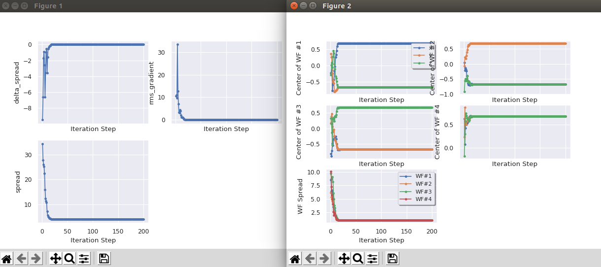
If AbiPy is installed on your machine, you can use the abiopen.py script
with the wout command and the --expose option to visualize the iterations
abiopen.py wannier90.wout --expose -sns
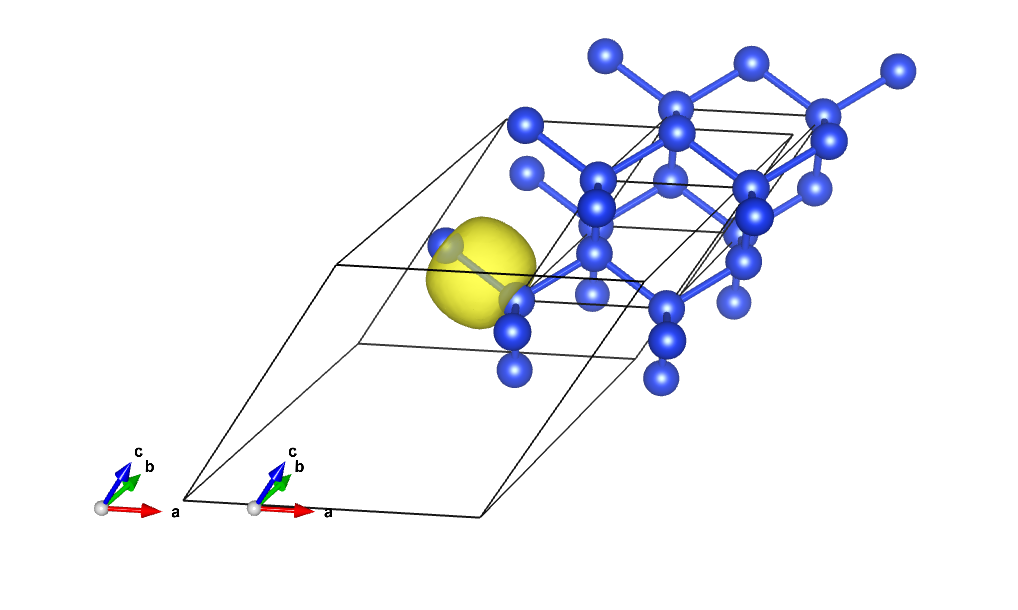
Visualize the Wannier functions
You can see the Wannier functions in XCrysDen format. Just type:
xcrysden --xsf wannier90_00001.xsf
To see the isosurface click on: Tools->Data Grid -> OK And modify the isovalue, put, for instance, 0.3 and check the option “Render ± isovalue” then click on OK Alternatively, one can read the xsf file with vesta . MacOsx users can use the command line:
open wannier90_00003.xsf -a vesta
to invoke vesta directly from the terminal:
Important
-
It is important to set istwfk equal to 1 for every k-point avoiding using symmetries. The reason is that the formalism used to extract the MLWF assumes that you have a uniform grid of k-points. See section IV of [Marzari1997].
-
The number of Wannier functions to extract should be minor or equal to the number of bands. If nband > nwan then the disentanglement routines will be called.
-
The number of k-points should be equal to ngkpt(1)*ngkpt(2)*ngkpt(3). This is achieved by using the input variables kptopt= 3, ngkpt and nshiftk= 1.
-
The prefix of all wannier90 files in this sample case is wannier90. Other possible prefixes are w90_ and abo __w90_ , where abo is the fourth line on your .file file. To setup the prefix, ABINIT will first look for a file named abo __w90.win_ if it is not found then it will look for w90.win and finally for wannier90.win.
3. The PAW case
Before starting it is assumed that you have already completed the tutorials PAW1 and PAW2.
For silicon, we just have to add the variable pawecutdg and the PAW Atomic Data is included in the pseudopotential file. An example has already been prepared.
Just copy the file tw90_2.abi into Work_w90:
cp ../tw90_2.abi .
We are going to reuse the wannier90.win of the previous example. Now, just run abinit again
abinit tw90_2.abi > log 2> err &
As it is expected, the results should be similar than those of the PW case.
Important
For the PAW case the UNK files are not those of the real wavefunctions. The contribution inside the spheres is not computed, however, they can be used to plot the Wannier functions.
4. Defining the initial projections
Up to now we have obtained the MLWF for the four valence bands of silicon. It is important to note that for valence states the MLWF can be obtained starting from a random initial position. However, for conduction states we have to give a very accurate starting guess to get the MLWF.
We are going to extract the \(sp^3\) hybrid orbitals of Silane SiH\(_4\). You can start by copying from the tests/tutoplugs directory the following files:
cp ../tw90_3.abi .
cp ../tw90_3o_DS2_w90.win .
Now run abinit
abinit tw90_3.abi > log 2> err &
While it is running, we can start to examine the input files. Open the main input file tw90_3.abi. The file is divided into three datasets.
#########################################################
# Silane SiH4
#########################################################

ndtset 2

#########################################################
# First dataset: SCF
#########################################################
  nstep1 200
 tolvrs1 1.0d-10
 kptopt1 1        # Option for the automatic generation of k points
 kptrlen1  20
 istwfk1 1      #Controls the form of the wavefunctions
 diemac 2
 prtden1 1   getden1 0   getwfk1 0    # Usual file handling data


#########################################################
# Second: Wannier90
#########################################################
     iscf2 -2      #non self-consistent field calculation
    nstep2 0       # zero steps, it will just read the previous wave function
   tolwfr2 1.e-20  #dummy here
   getwfk2 1       # Get wavefunction of dataset 1
   getden2 1       # Get density file of dataset 1
   istwfk2 8*1     # Controls the form of the wavefunctions
   kptopt2 3       # Option for the automatic generation of k points
    nband2 4
#wannier90 related variables
  prtwant2 2      # keyword for a wannier90 calculation
w90prtunk2 1      # print UNK files
w90iniprj2 2      # initial projections are defined in wannier90.win

#########################################################
# Data common to all datasets
#########################################################

#kpoint grid
  ngkpt2 2 2 2     # 2*2*2 kpoints in the full Brillouin zone
                   # we need a homogeneous grid to get the Wannier functions
                   #
nshiftk2 1
 shiftk2 0.0 0.0 0.0

#Definition of the unit cell
#Molecule: 9.36 in x, 7.0104 in and 0.1 in z (Bohrs)
acell 12 12 12  #12 Bohrs
rprim  1.0  0.0  0.0
       0.0  1.0  0.0
       0.0  0.0  1.0

#Definition of the atom types
ntypat 2
znucl 14 1

# enforce calculation of forces at each SCF step
 optforces 1

#Definition of the atoms
natom 5
typat 1 2 2 2 2
xcart
    0.00000000E+00    0.00000000E+00    0.00000000E+00
    0.19965920E+01    0.19965920E+01    0.19965920E+01
    0.19965920E+01   -0.19965920E+01   -0.19965920E+01
   -0.19965920E+01    0.19965920E+01   -0.19965920E+01
   -0.19965920E+01   -0.19965920E+01    0.19965920E+01


#Definition of the planewave basis set
ecut  8       # Maximal kinetic energy cut-off, in Hartree
              # This is too low too


 pp_dirpath "$ABI_PSPDIR"
 pseudos "Psdj_nc_sr_04_pw_std_psp8/Si.psp8, Psdj_nc_sr_04_pw_std_psp8/H.psp8"

##############################################################
# This section is used only for regression testing of ABINIT #
##############################################################
#%%<BEGIN TEST_INFO>
#%% [setup]
#%% executable = abinit
#%% [shell]
#%% pre_commands =
#%%    iw_cp tw90_3o_DS2_w90.win tw90_3o_DS2_w90.win
#%% [files]
#%% files_to_test =
#%%  tw90_3.abo,  tolnlines=   12,   tolabs=  3.00e-04,   tolrel=  2.00e-02, fld_options = -medium
#%% extra_inputs =
#%% [paral_info]
#%% max_nprocs = 1
#%% [extra_info]
#%% authors = Unknown
#%% keywords = NC
#%% description = Silane SiH4. Generation of Wannier functions via Wannier90 code.
#%%<END TEST_INFO>
First a SCF calculation is done. What follows is a NSCF calculation including more bands. Finally, in the third dataset we just read the wavefunction from the previous one and the Wannier90 library is called. w90iniprj is a keyword used to indicate that the initial projections will be given in the .win file.
Note
You may notice that the .win file is now called tw90_3o_DS2_w90.win. It has the following form: prefix_dataset_w90.win, where the prefix is taken from the third line of your .file file. and dataset is the dataset number at which you call Wannier90 (dataset 2 in this example).
Now open the .win file. The initial projections will be the \(sp^3\) hybrid orbitals centered in the position of the silicon atom. This is written explicitly as:
begin projections
Si:sp3
end projections
There is an enormous freedom of choice for the initial projections. For instance, you can define the centers in Cartesian coordinates or rotate the axis. Please refer to the Wannier90 user guide and see the part related to projections (see www.wannier90.org).
5. More on Wannier90 + ABINIT
Now we will redo the silicon case but defining different initial projections.
This calculation will be more time consuming, so you can start by running the calculation while reading:
cp ../tw90_4.abi .
cp ../tw90_4o_DS3_w90.win .
abinit  tw90_4.abi > log 2> err &
Initial projections:
In this example we extract sp\(^3\) orbitals centered on the silicon atoms. But you could also extract bonding and anti-bonding orbitals by uncommenting and commenting the required lines as it is indicated in tw90_4o_DS3_w90.win.
You can see that we are using r=4 in the initial projections block. This is to indicate that the radial part will be a Gaussian function whose width can be controlled by the value of the variable zona. The main advantage over radial functions in the form of hydrogenic orbitals is that the time to write the .amn file will be reduced.
Interpolated band structure
We are going to run Wannier90 in standalone mode. Just comment out the following lines of the .win file:
postproc_setup = .true.   !used to write .nnkp file at first run
num_iter = 100
And uncomment the following two lines:
!restart = plot
!bands_plot = .true.
Now run Wannier90:
$ABI_HOME/fallbacks/exports/bin/wannier90.x-abinit tw90_4o_DS3_w90
The interpolated band structure is in tw90_4o_DS3_w90_band.dat
To plot the bands, open gnuplot in the terminal and type:
gnuplot "tw90_4o_DS3_w90_band.gnu"
6. A second example: La2CuO4
As a next example, we will compute a single MLWF for the cuprate La2CuO4. This material is the parent compound of a set of non-conventional superconductors. DFT predicts it is a metal, yet experimentally it is a well known antiferromagnetic insulator. The reason is that it is a strongly correlated material which undergoes a Mott transition.
Because DFT with the LDA functional is not able to account for strong electronic correlations, one needs to use many-body methods to correctly describe the insulating phase of this material. For example, one can apply DFT+DMFT to describe the Mott transition correctly.
In this tutorial, we will show how one can construct an effective Hamiltonian in the correlated orbital subset using Wannier90. Once this Hamiltonian is generated, DMFT can be applied to study the Mott transition.
6.1 Orbital characters of the band structure
Let’s start by running the first calculations. Copy this file:
cp ../tw90_5.abi .
and run abinit using
mpirun -n 4 abinit tw90_5.abi > tw90_5.log &
This calculation should take a couple of minutes.
The most important physics at low energy derives from the orbitals near the Fermi level. In order to correctly select the subset of correlated orbitals that we want to model in our effective Hamiltonian and how to project it, we need to study the orbital character of the band structure of the material.
Let’s look at the input file:
#############################################################################
# La2CuO4 : Fatbands
#############################################################################

#############################################################################
# Structural parameters
#############################################################################
acell            3*1

rprim            3.6077606084241   3.6077606084241  -12.478046911766
                -3.6077606084241   3.6077606084241   12.478046911766
                 3.6077606084241  -3.6077606084241   12.478046911766

natom            7
ntypat           3
typat            1 1 2 3 3 3 3
znucl            57 29 8
xcart            0.0000000000  0.0000000000  9.0145301354
                 3.6077606086  3.6077606086  3.4635167757
                 0.0000000000  0.0000000000  0.0000000000
                 0.0000000000  3.6077606086  0.0000000000
                 3.6077606086  0.0000000000  0.0000000000
                 0.0000000000  0.0000000000  4.6340316725
                 3.6077606086  3.6077606086  7.8440152387

# Two datasets: Ground state and Fatbands
ndtset           2
jdtset           1 2

# Shared parameters
nband            38
nbdbuf           4     # Extra bands easing convergence
ecut             10    # Low but sufficient
pawecutdg        18    # Low but sufficient
occopt           3     # Metal with partially occupied orbitals
tsmear           0.01  # Effective temperature

pawprtvol        3

nstep            100
nline            3
nnsclo           3
tolwfr           1.0e-6
istwfk          *1

#############################################################################
# First dataset: Ground state
#############################################################################
ngkpt1           6 6 6       # Coarse but sufficient
nshiftk1         1
shiftk1          0.5 0.5 0.5

#############################################################################
# Second dataset: Fatbands for orbital characters
#############################################################################
getden2         -1       # Use density of the previous dataset
nshiftk2         1
shiftk2          0 0 0   # Non shifted grid
# nbandkss2        2
# kssform2         3
pawfatbnd2       2       # Fatbands resolved in L and M
pawprtdos2       2       # Useful for abipy
prtdos2          3       # Useful for abipy
prtdosm2         2       # Useful for abipy
iscf2           -2       # Non-self-consistent calculation
kptopt2         -4       # Four paths in the band structure
ndivk2           10 10 12 3   # Divisions for each paths
kptbounds2       0.00000000  0.00000000  0.00000000     # Paths
                 0.27456608  0.27456608 -0.27456608
                 0.50000000  0.00000000  0.00000000
                 0.00000000  0.00000000  0.00000000
                -0.25000000  0.25000000  0.25000000

pp_dirpath       "$ABI_PSPDIR"
pseudos          "Psdj_paw_pw_std/La.xml, Psdj_paw_pw_std/Cu.xml, Psdj_paw_pw_std/O.xml"


##############################################################
# This section is used only for regression testing of ABINIT #
##############################################################
#%%<BEGIN TEST_INFO>
#%% [setup]
#%% executable = abinit
#%% [paral_info]
#%% max_nprocs = 4
#%% nprocs_to_test = 4
#%% [NCPU_4]
#%% files_to_test =
#%%    tw90_5_MPI4.abo, tolnlines=5, tolabs=7.00e-05, tolrel=1.10e+00, fld_options=-medium
#%% [extra_info]
#%% authors = O. Gingras
#%% keywords = PAW
#%% description = Test interface with Wannier90 (PAW pseudopotentials)
#%%<END TEST_INFO>
#
The first dataset is simply useful to compute the ground state. DFT will predict it to be metallic, so we use an occupation option occopt for metals.
In the second dataset, we compute a band structure along with the orbital character of the bands. We use pawfatbnd to specify that we want the L and M resolved orbitals, meaning we want to separate the contributions for the angular momentum L and its projection M. We select a high symmetry path using kptbounds. A few parameters are useful for the postprocessing step following, that is pawprtdos, prtdos and prtdosm.
Now before looking at the output from the calculation, let’s discuss what we expect to find. The correlated atom here is the cupper, which has a partially filled 3d shell. The d means the orbitals have angular momentum l=2. There are 5 such orbitals, with two spins.
In vaccuum, these 10 states are degenerate. However, La2CuO4 here has a layered perosvkite structure, which means the cupper atom feels a crystal field produced by the surrounding atoms. In particular, an octaedron of oxygen with lift the degeneracy of the 3d shell into two subshells: the t2g and eg shells. Furthermore, the elongation of this octaedron splits even more these subshells. The resulting splits are illustrated in the following figure.

Additionally, by counting the stoechiometry of this material, we find that there should be 9 electrons occupying this shell, thus we expect only the x2-y2 orbital to be partially filled, at the Fermi level.
Tip
Let’s now look at the resulting fatbands now. We use abipy with the following commands in a python script:
from abipy.abilab import abiopen

with abiopen("tw90_5o_DS2_FATBANDS.nc") as fb:
    fb.plot_fatbands_mview(iatom=2, fact=1.5, lmax=2, ylims=[-8, 2])
These are the fatbands for the atom 2 (third atom as python starts at 0), thus the cupper atom. First column is the s character, second are the 3 p characters and last column are the 5 d characters. The last one is the dx2-y2, the only one that is partially filled, as expected.
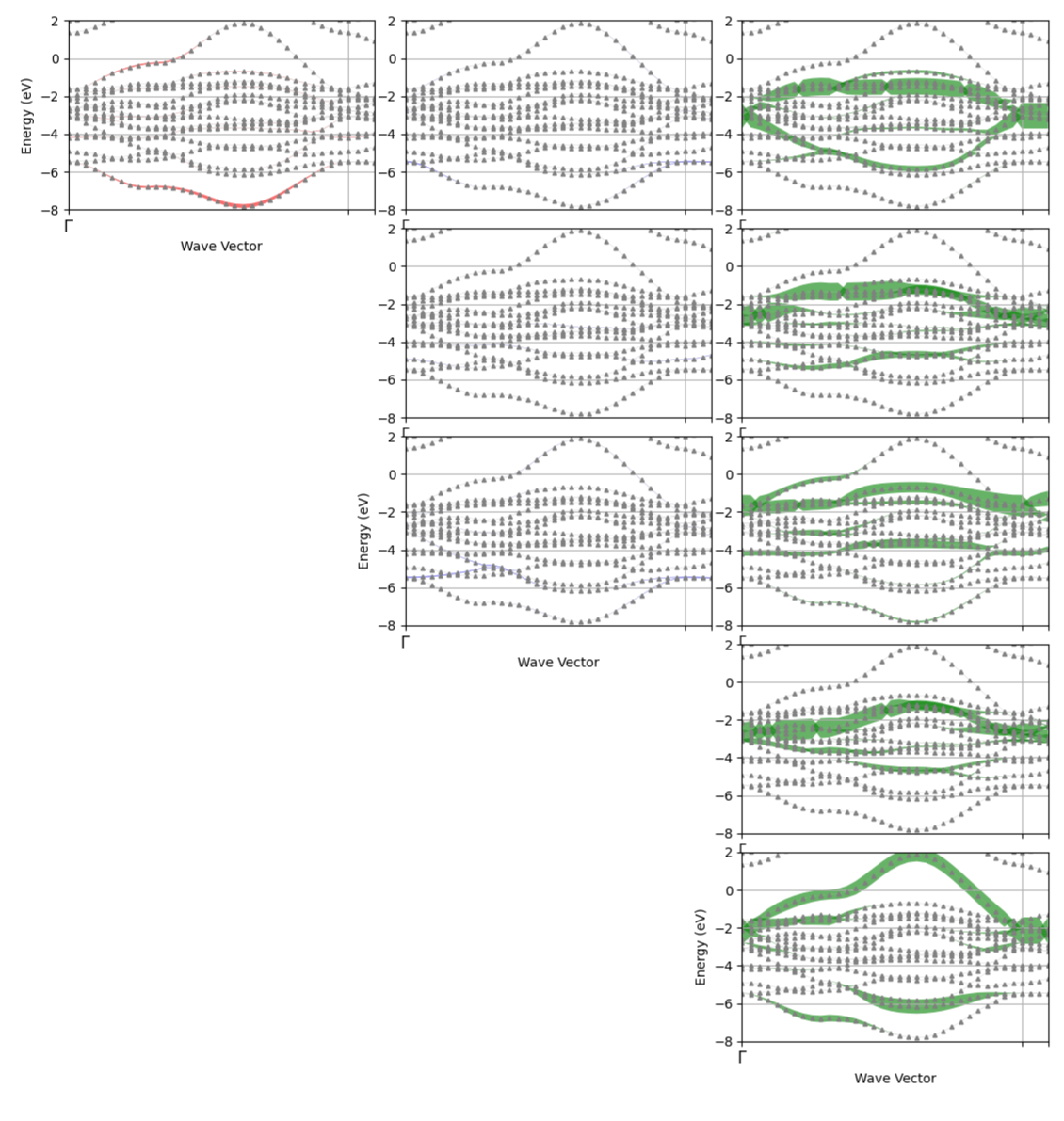
This block contains 17 bands, mostly formed by the hybridization of the 4 times 3 O-2p orbitals with the 5 Cu-3d orbitals. It includes band numbers 19 to 33.
6.2 Wannier90 projection
We will now use the ABINIT + Wannier90 interface to compute an effective Hamiltonian for the Cu 3d x^2 -y^2 orbital. First copy this file:
cp ../tw90_6.abi .
cp ../tw90_6o_DS3_w90.win .
and run abinit using
mpirun -n 4 abinit tw90_6.abi > tw90_6.log &
This calculation should take a couple of minutes. It uses two files. The first one is
#############################################################################
# La2CuO4: Wannier90
#############################################################################
# Structural parameters
#############################################################################
acell            3*1

rprim            3.6077606084241   3.6077606084241  -12.478046911766
                -3.6077606084241   3.6077606084241   12.478046911766
                 3.6077606084241  -3.6077606084241   12.478046911766

natom            7
ntypat           3
typat            1 1 2 3 3 3 3
znucl            57 29 8
xcart            0.0000000000  0.0000000000  9.0145301354
                 3.6077606086  3.6077606086  3.4635167757
                 0.0000000000  0.0000000000  0.0000000000
                 0.0000000000  3.6077606086  0.0000000000
                 3.6077606086  0.0000000000  0.0000000000
                 0.0000000000  0.0000000000  4.6340316725
                 3.6077606086  3.6077606086  7.8440152387

# Four datasets: Ground state on coarse grid, non-self-consistent calculations on
# finer grid, wannier90 projection, band structure
ndtset           4

# Shared parameters
nband            38    # Number of bands
nbdbuf           4     # Extra bands easing convergence
ecut             10    # Low but sufficient
pawecutdg        18    # Low but sufficient

nshiftk          1     # For most datasets, need no shift
shiftk           0 0 0

#############################################################################
# First dataset: Ground state on a coarse grid
#############################################################################
ngkpt1           6 6 6
shiftk1          0.5 0.5 0.5
nstep1           100
tolvrs1          1.0d-8
prtden1          1     # Print density for other datasets
prtwf1           1
diemac1          12.0
istwfk1         *1

#############################################################################
# Second dataset: Non-self-consistent ground state on a finer grid
#############################################################################
iscf2           -2
prtvol2          1
nstep2           100
tolwfr2          1e-9   # Good resolution on the wave function necessary
getwfk2          1      # Get wave function and density from previous dataset
getden2          1
prtden2          1      # Print for next one
prtwf2           1
ngkpt2           8 8 8

#############################################################################
# Third dataset: Call to the Wannier90 library
#############################################################################
prtvol3          1
iscf3           -2
nstep3           0
tolwfr3          1e-9
getwfk3          2
getden3          2
prtwant3         2     # ABINIT - Wannier90 interface
istwfk3         *1
kptopt3          3     # Do not use symmetries
ngkpt3           8 8 8
w90prtunk3       0     # Do not prints the unk matrices
w90iniprj3       2     # Use projection defined in the .win file

#############################################################################
# Fourth dataset: Band structure on the same path as Wannier90
#############################################################################
iscf4           -2
getden4         -2
getwfk4         -2
kptopt4         -4    # Four segments of paths
ndivsm4          13    # Smallest path has 16 points, other scaled
kptbounds4       0.00000000  0.00000000  0.00000000  # Gamma
                 0.25000000  0.25000000 -0.25000000  # Sigma
                 0.50000000  0.00000000  0.00000000  # X
                 0.00000000  0.00000000  0.00000000  # Gamma
                -0.25000000  0.25000000  0.25000000  # Z
tolwfr4          1.0d-9
enunit4          1

pp_dirpath       "$ABI_PSPDIR"
pseudos          "Psdj_paw_pw_std/La.xml, Psdj_paw_pw_std/Cu.xml, Psdj_paw_pw_std/O.xml"


##############################################################
# This section is used only for regression testing of ABINIT #
##############################################################
#%%<BEGIN TEST_INFO>
#%% [setup]
#%% executable = abinit
#%% [shell]
#%% pre_commands = iw_cp tw90_6o_DS3_w90.win tw90_6_MPI4o_DS3_w90.win
#%% [paral_info]
#%% max_nprocs = 4
#%% nprocs_to_test = 4
#%% [NCPU_4]
#%% files_to_test =
#%%    tw90_6_MPI4.abo, tolnlines=5, tolabs=7.00e-05, tolrel=1.10e+00, fld_options=-medium
#%% [extra_info]
#%% authors = O. Gingras
#%% keywords = wannier90, PAW
#%% description = Test interface with Wannier90 (PAW pseudopotentials)
#%%<END TEST_INFO>
which contains four datasets. In the first one, we simply compute the density and wave function of the ground state on a coarse grid. In the second dataset, we use this coarse-grid ground state to do a non-self-consistent calculation on a finer grid. In the third dataset, we call the Wannier90 library to perform the projection, which uses the data computed in the second dataset. The fourth dataset computes a band structure, that we use to compare with the projected band structure computed by Wannier90.
The important part here happens in the third set. The Wannier90 library uses the following input file:
num_wann = 1
num_bands = 38

begin projections
 Cu:dx2-y2
end projections

write_hr = true
guiding_centres = true
postproc_setup = true

exclude_bands = 1-28, 34-38
dis_win_min = 4
dis_win_max = 8.5
dis_froz_min = 6
dis_froz_max = 8.5
dis_num_iter = 1000
dis_conv_tol = 1e-11

num_iter = 1000
conv_tol = 1e-11

bands_plot = true
begin kpoint_path
 G  0.00  0.00  0.00  N  0.25  0.25 -0.25
 N  0.25  0.25 -0.25  X  0.50  0.00  0.00
 X  0.50  0.00  0.00  G  0.00  0.00  0.00
 G  0.00  0.00  0.00  M -0.25  0.25  0.25
end kpoint_path
bands_num_points = 20
The keywords can be understood using Wannier90’s user guide found on their web page (https://raw.githubusercontent.com/wannier-developers/wannier90/v3.1.0/doc/compiled_docs/user_guide.pdf).
We want to make a one band model of the dx^2 -y^2 cupper orbital, which is defined by the projection keyword. As seen from the fatbands calculation, this orbital has overlap with many bands, across a specific energy window. The non-important bands which can give a non-accurate representation of the band structure are excluded using the exclude_bands keyword. The energy window is defined using the dis_win_min and dis_win_max keywords.
Moreover, this orbital has to be disentangled with other orbital, so we need the disentanglement procedure. The number of iterations in specified by dis_num_iter.
Finally, we want to compare the resulting band structure with the one coming from the Kohn-Sham basis. This is enforced using the bands_plot keyword, along with a defined path which corresponds to the same path as the one calculated in ABINIT.
To plot the resulting band structures, you will need a little bit of work. Run this python script:
python ../EIG_to_col.py
Then you can use gnuplot to plot both the band structures together to compare them, with something like:
echo 'plot [][0:9] "tw90_6o_DS3_w90_band.dat" u ($1/3.0470170):2 tit "Wannier90" w l lw 4, "band_struct.dat" u ($1/167):2 tit "DFT" w l
pause -1' > plot.gnu
gnuplot plot.gnu
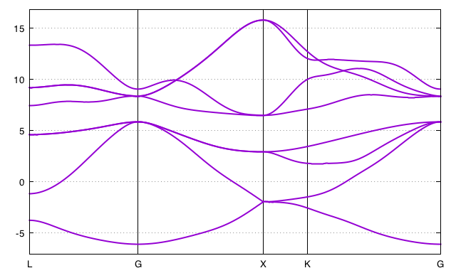
Performing the calculation with more converged parameters, we find the following band strcture:
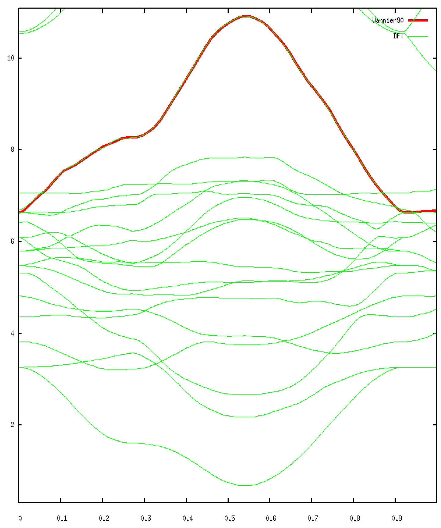
The resulting Hamiltonian is written as the tw90_6o_DS3_w90_hr.dat file. It can be used for example using the TRIQS package to apply DMFT, thus correcting the DFT calculation to compute correctly the strong electronic correlations. We would then observe a Mott transition with respect to temperature.
7. Run ABINIT-Wannier90 in post-processing mode with the example of GaAs
Now we use ABINIT-Wannier90 in the post-processing mode to construct the Wannier functions for GaAs.
cp ../tw90_7.abi .
cp ../tw90_7o_DS2_w90.win .
In this mode, we can do the SCF calculation in the first dataset with the kpoints in IBZ. Then we run post-processing in the second dataset, which reads the wavefunction generated in the first dataset, use symmetry to get the wavefunction in FBZ, and compute the Wannier functions from that. The first dataset is just the usual SCF input. In the second dataset, there is:
 optdriver2 8
 wfk_task2 "wannier"
 getwfk2   -1   # Read WKF in the IBZ from first dataset.
 prtwant2 2
 w90iniprj2 2
where optdrive 8 means that it is a post-processing of the WFK file, and wfk_task wannier tells that the ABINIT-Wannier interface will be executed. The other options are the same as in the “single-run” mode. And we also need to provide the Wannier90 “.win” input file, which is also the same as in the “single-run” mode. In this mode, we use the same kpoint options as the SCF run (first dataset) instead of specifying the options for generating the k-points for the FBZ, as the wavefunction for the FBZ is automatically generated.
After running the command:
abinit tw90_7.abi > tw90_7.log 2> tw90_7.err
we get the usual output of the ABINIT-Wannier run, including the “.amn”, “.mmn” files, and so on.