First tutorial on MULTIBINIT

Build a second-principles effective atomistic model and run finite-temperature lattice dynamics simulations

This lesson aims at learning how to build an effective atomistic model from a set of first-principles data and then use it for simulations at finite temperatures.

Before beginning, it is very important to read the reference [Wojdel2013].

Within this lesson, we will describe :

• the complete set of first-principles data to be provided.
• the steps for constructing a model for a prototypical compound (BaHfO$_3$).
• the way to perform a finite temperature simulation from the previous model.

In this tutorial, we make the hypothesis that you have already acquired a practical knowledge regarding Density Functional Theory (DFT) and Density Functional Perturbation Theory (DFPT). In particular, DFPT is a key feature of ABINIT directly exploited by MULTIBINIT. In order to learn how to use the DFPT (producing the related DDB) and the associated code to merge different DDB files, please have a look at the tutorials on phonon response, strain response and mrgddb. After these tutorials, you should be able to perform a full DFPT calculation in order to produce DDB file. In this tutorial will not provide the inputs for ABINIT DFPT calculations (that you can be found in the previously cited tutorials) but instead the final DDB resulting from them.

Tips

Note: The models generated in this tutorial are not supposed to be used in production.

The AGATE software is also required for this tutorial, as a tool for the analysis of the results. You can install it on debian with:

sudo add-apt-repository ppa:piti-diablotin/abiout
sudo apt-get update && sudo apt-get install abiout

Note

Supposing you made your own installation of ABINIT, the input files to run the examples are in the ~abinit/tests/ directory where ~abinit is the absolute path of the abinit top-level directory. If you have NOT made your own install, ask your system administrator where to find the package, especially the executable and test files.

In case you work on your own PC or workstation, to make things easier, we suggest you define some handy environment variables by executing the following lines in the terminal:

export ABI_HOME=Replace_with_absolute_path_to_abinit_top_level_dir # Change this line
export PATH=$ABI_HOME/src/98_main/:$PATH      # Do not change this line: path to executable
export ABI_TESTS=$ABI_HOME/tests/             # Do not change this line: path to tests dir
export ABI_PSPDIR=$ABI_TESTS/Psps_for_tests/  # Do not change this line: path to pseudos dir

Examples in this tutorial use these shell variables: copy and paste the code snippets into the terminal (remember to set ABI_HOME first!) or, alternatively, source the set_abienv.sh script located in the ~abinit directory:

source ~abinit/set_abienv.sh

The ‘export PATH’ line adds the directory containing the executables to your PATH so that you can invoke the code by simply typing abinit in the terminal instead of providing the absolute path.

To execute the tutorials, create a working directory (Work*) and copy there the input files of the lesson.

Most of the tutorials do not rely on parallelism (except specific tutorials on parallelism). However you can run most of the tutorial examples in parallel with MPI, see the topic on parallelism.

1 Method and first-principles inputs

As described in [Wojdel2013], the construction of a lattice model with MULTIBINIT consists in determining an explicit form of the Born-Oppenheimer (BO) energy surface around a reference structure (RS), in terms of individual atomic displacements $\boldsymbol{u}$ and macroscopic strains $\boldsymbol{\eta}$ :

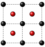
Fig. 1: Example of cubic RS made by two different (black and red) atomic species.

$$\displaystyle E^{tot}(\boldsymbol{u},\boldsymbol{\eta}) = E^{0} + E^{phonon}(\boldsymbol{u}) + E^{elastic}(\boldsymbol{\eta}) + E^{coupling}(\boldsymbol{u},\boldsymbol{\eta})$$

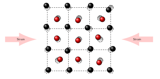
Fig. 2: Example of lattice perturbations: atomic displacements and strain.

The methodology followed in MULTIBINIT consists in making a Taylor expansion around the RS, which is assumed to be a stationary point of the BO energy surface. As such, the energy expression can be further decomposed as follows :

$$\displaystyle E^{tot}(\boldsymbol{u},\boldsymbol{\eta}) = E^{0} + [ E^{phonon}_{harm}(\boldsymbol{u}) + E^{elastic}_{harm}(\boldsymbol{\eta}) + E^{coupling}_{harm}(\boldsymbol{u},\boldsymbol{\eta})] + [E^{phonon}_{anharm}(\boldsymbol{u}) + E^{elastic}_{anharm}(\boldsymbol{\eta}) + E^{coupling}_{anharm}(\boldsymbol{u},\boldsymbol{\eta})]$$

The first term $E^0$ is the energy of the RS, which has been fully relaxed (e.g. ionmov=2 and optcell=2) with very strict tolerance criterium (tolmxf < 1E-7) since we assume that all first energy derivatives are zero. This $E^0$ energy has to be included in the global DDB file, by including the ground-state DDB when merging all partial DDBs with mrgddb.

Then, for the set of harmonic terms, the coefficients correspond to various second derivatives of the energy respect to atomic displacements and macroscopic strains. They can be directly computed with ABINIT using DFPT (phonon response, strain response) and used as parameters of our model. See also electric polarization. As such, our second-principles model reproduces exactly the first-principles results at the harmonic level (i.e. full phonon dispersion curves, elastic and piezoelectric constants of the RS). In practice, the global DDB file produced by ABINIT is so used as an input file for MULTIBINIT containing all the harmonic coefficients.
This file must contain second energy derivatives respect to (i) all atomic displacements (rfphon 1; rfatpol 1 natom; rfdir 1 1 1) on a converged grid of q-points (defining the range of interactions in real space), (ii) macroscopic strains (rfstrs 3; rfdir 1 1 1) and also, for insulators, (iii) electric fields (rfelfd 1; rfdir 1 1 1) in order to provide the Born effective charges and dielectric constant used for the description of long-range dipole-dipole interactions.

The coefficients of the set of anharmonic terms correspond to higher-order derivatives of the energy respect to atomic displacements and macroscopic strains. They are numerous and not computed individually at the first-principles level. Instead, the most important terms will be selected by MULTIBINIT and related coefficients fitted in order to reproduce the BO energy surface. To that end, a training set (TS) of ABINIT data needs to be provided on which the fit will be realized. This TS consists in a set of atomistic configurations realized on a suitable supercell depending on the range of anharmonic interactions (typically 2x2x2 supercell) and for which energy, forces and stresses are provided. This takes the form of an ABINIT netcdf “_HIST.nc” file. Providing an appropriate TS, properly sampling the BO surface, is crucial to obtain an appropriate model. How to built it depends on the kind of system (stable or with instabilities) and will not be further discussed here.

In summary, constructing a second-principles lattice model with MULTIBINIT requires two input files which are direct output of ABINIT : (i) a full “DDB” file containing the reference energy and second energy derivatives which correspond to harmonic coefficients of the model and (ii) a “_HIST.nc” file containing the energy, forces and stresses of an appropriate training set of configurations from which the anharmonic terms will be automatically selected and fitted.

For this tutorial both these files will be provided.

2 Fitting procedure: creating anharmonicities

In this tutorial, we take the perovskite $\mathrm{BaHfO_3}$ in its cubic phase as an exemple of a material without lattice instabilities.

Optional exercise $\Longrightarrow$ Compute the phonon band structure with anaddb.

You can download the complete DDB file (resulting from the previous calculations) here:

View tests/tutomultibinit/Input/tmulti_l_6_DDB

Before starting, you might to consider working in a different subdirectory than for the other lessons. Why not create “Work_fitLatticeModel”?

The file “~abinit/tests/tutomultibinit/Input/tmulti_l_6_1.files” lists the file names and root names. You can copy it in the Work_fitLatticeModel directory and look at this file content, you should see:

  tmulti_l_6_1.abi
  tmulti_l_6_1.abo
  tmulti_l_6_DDB
  no
  tmulti_l_6_HIST.nc
  no

As mentioned in the guide of MULTIBINIT:

• “tmulti_l_6_1.abi” is the main input file
• “tmulti_l_6_1.abo” is the main output file
• “tmulti_l_6_DDB” is the DDB which contains the system definition and the list of energy derivatives
• “tmulti_l_6_HIST.nc” is the set of DFT configurations to fit

It is now time to copy the file ~abinit/tests/tutomultibinit/Input/tmulti_l_6_1.abi, ~abinit/tests/tutomultibinit/Input/tmulti_l_6_DDB and tmulti_l_6_HIST.nc in your Work_fitLatticeModel directory. You should read carefully the input file:

View tests/tutomultibinit/Input/tmulti_l_6_1.abi

and read the documentation about the fit input variables:

• fit_ncoeff
• fit_rangepower
• fit_cutoff
• fit_spc_maxs
• fit_iatom
• fit_efs
• sel_efs

You can now run (it should take less than 2 minutes):

mpirun -np 10 multibinit < multi_l_6_1.files > tmulti_l_6_1_stdout&

The resulting output file “tmulti_l_6_1.abo” should be rather similar to the one below.

View tests/tutomultibinit/Refs/tmulti_l_6_1.abo

The fitted anharmonocites are stored in “tmulti_l_6_1_coeffs.xml” and informations about the differences between the DFT data and the model are stored in “TRS_fit_diff_energy.dat” and “TRS_fit_diff_stress.dat”. The global information about the reproduction of the DFT data is written in the output file.

Before the fit (including the harmonic part only), the goal function is equal to:

Goal function values at the begining of the fit process (eV^2/A^2):
    Energy          :   2.2780100662032291E-03
    Forces+Stresses :   3.9733621903060741E-02
    Forces          :   2.4711894644538119E-02
    Stresses        :   1.5021727258522627E-02

After adding the anharmonicities, the goal function value is equal to

Goal function values at the end of the fit process (eV^2/A^2):
    Energy          :   1.7493658081925374E-04
    Forces+Stresses :   1.1685294481702690E-02
    Forces          :   9.1861216904870410E-03
    Stresses        :   2.4991727912156494E-03

In order to save computational time, the previous example restricts the fitting procedure to fit_iatom = 2. This means that only anharmonic terms linked to the interactions between Hf and its nearest neighbours are considered, which might not be enough to produce a fully accurate model.

Optional exercise $\Longrightarrow$ Try to fit on all irreducible atoms with fit_iatom = 0. This procedure is time consumming (around 15 min). You can also play with fit_cutoff to see if there is other terms selected.

3 Bounding of the model

Since the approach of the procedure is based on a polynomial expansion of the energy, it is common that the produced model is diverging at high temperature. In order to avoid this divergence, we will produce additional terms (order 6 and 8 terms) that ensure the boundness of the model.

Before starting, you might to consider working in a different subdirectory than for the other lessons. Why not create “Work_boundingLatticeModel”?

The file ~abinit/tests/tutomultibinit/Input/tmulti_l_7_1.files lists the file names and root names. You can copy it in the Work_boundingLatticeModel directory and look at this file content, you should see:

  tmulti_l_7_1.abi
  tmulti_l_7_1.abo
  tmulti_l_6_DDB
  tmulti_l_7_1_coeffs.xml
  tmulti_l_6_HIST.nc
  no

“tmulti_l_7_1_coeffs.xml” is the model that we produced with fit_iatom=0 and fit_cutoff=$a \sqrt{3}/2$ and has to be bounded.

It is now time to copy the file ~abinit/tests/tutomultibinit/Input/tmulti_l_7_1.abi, ~abinit/tests/tutomultibinit/Input/tmulti_l_6_DDB, tmulti_l_7_1_coeffs.xml and tmulti_l_6_HIST.nc in your Work_boundingLatticeModel directory. You should read carefully the input file:

View tests/tutomultibinit/Input/tmulti_l_7_1.abi

and read the documentation about the bounding input variables:

• bound_model
• bound_rangepower
• bound_penalty

You can now run (it should take less than 1 minute):

multibinit < multi_l_7_1.files > tmulti_l_7_1_stdout&

After this procedure, a new model has been generated with higher-order even terms according to bound_rangepower. You can check in the ouput file that the inclusion of these new terms preserves the value of the goal function for forces and stresses.

4 Running molecular dynamics with an effective model

The aim of the construction of effective models is to be able to run realistic molecular-dynamics simulations in order to access material properties at finite temperatures.

The file ~abinit/tests/tutomultibinit/Input/tmulti_l_8_1.files lists the file names and root names. You can copy it in the Work_MDLatticeModel directory and look at this file content, you should see:

  tmulti_l_8_1.abi
  tmulti_l_8_1.abo
  tmulti_l_6_DDB
  tmulti_l_8_1.xml
  no
  no

“tmulti_l_8_1_coeffs.xml” is the model that have been bounded in the previous step.

It is now time to copy the file ~abinit/tests/tutomultibinit/Input/tutomulti_l_7_1.abi, ~abinit/tests/tutomultibinit/Input/tmulti_l_6_DDB, tmulti_l_7_1_coeffs.xml and tmulti_l_6_HIST.nc in your Work_MDLatticeModel directory. You should read carefully the input file:

View tests/tutomultibinit/Input/tmulti_l_8_1.abi

and read the documentation about the fit input variables:

• dynamics
• hmctt
• ntime
• dtion

You can now run (it should take less than 2 minutes):

multibinit -np 10 < multi_l_8_1.files > tmulti_l_8_1_stdout&

You can visualize your dynamics with the AGATE software:

agate tmulti_l_8_1_HIST.nc

This simulation intents to reproduce the behaviour of BaHfO$_\mathrm{3}$ at room temperature. You can check that the system is thermalized at the end of the calculation by looking at energergy, pressure, volume and temperature with the AGATE software:

• :plot etotal
• :plot P
• :plot V
• :plot T

$\mathrm{BaHfO_3}$ remains cubic at all temperatures which is not the case of all materials. For instance, $\mathrm{SrTiO_3}$ exhibits an antiferrodistrotive (AFD) phase transition from $\mathrm{Pm\bar{3}m}$ to $\mathrm{I4/mcm}$ at 105K (experimentally). MULTIBINIT allows to study such kind of structural phase transition.

Optional exercise $\Longrightarrow$ Try to recover the phase transition of $\mathrm{SrTiO_3}$ (PBEsol DDB is located in “~abinit/tests/tutomultibinit/Input/tutomulti_l_9_1.ddb” and the anharmonic part of the model in “~abinit/tests/tutomultibinit/Input/tmulti_l_9_1.xml”).

You should recover the results above, which highlights properly the AFD phase transition although at slightly higher temperature than experimentally observed. You should also notice the appeaance of polarization at very low temperature: this arises from the incipient ferroelectric character of $\mathrm{SrTiO_3}$ using classical MD simulations, neglecting quantum fluctuations.

---

This MULTIBINIT tutorial is now finished.