Parallelism in the DFPT formalism
Atomic displacements, homogeneous electric fields, strain.
This tutorial aims at showing how to use the parallelism for all the properties that are computed on the basis of the density-functional perturbation theory (DFPT) part of ABINIT, i.e.:
- responses to atomic displacements (to compute phonon frequencies, band structures, … )
- responses to homogeneous electric fields (dielectric constant, Born effective charges, Infra-red characteristics )
- responses to strain (elastic constants, piezoelectric constants …)
Such computations are realized when one of the input variables rfphon, rfelfd or rfstrs are non-zero, which activates optdriver=1. You are supposed to be well-familiarized with such calculations before starting the present tutorial. See the respfn help file, the input variables described in dfpt varset and the tutorial Response-Function 1 and subsequent tutorials.
You will learn about the basic implementation of parallelism for DFPT calculations, then will execute a very simple, quick calculation for one dynamical matrix for FCC aluminum, whose scaling is limited to a few dozen computing cores, then you will execute a calculation whose scaling is much better, but that would take a few hours in sequential, using a provided input file.
For the last section of that part, you would be better off having access to more than 100 computing cores, although you might also change the input parameters to adjust to the machine you have at hand. For the other parts of the tutorial, a 16-computing-core machine is recommended, in order to perform the scalability measurements.
You are supposed to know already some basics of parallelism in ABINIT, explained in the tutorial A first introduction to ABINIT in parallel.
This tutorial should take less than two hours to be done if a powerful parallel computer is available.
Note
Supposing you made your own installation of ABINIT, the input files to run the examples are in the ~abinit/tests/ directory where ~abinit is the absolute path of the abinit top-level directory. If you have NOT made your own install, ask your system administrator where to find the package, especially the executable and test files.
In case you work on your own PC or workstation, to make things easier, we suggest you define some handy environment variables by executing the following lines in the terminal:
export ABI_HOME=Replace_with_absolute_path_to_abinit_top_level_dir # Change this line
export PATH=$ABI_HOME/src/98_main/:$PATH      # Do not change this line: path to executable
export ABI_TESTS=$ABI_HOME/tests/             # Do not change this line: path to tests dir
export ABI_PSPDIR=$ABI_TESTS/Pspdir/  # Do not change this line: path to pseudos dir
Examples in this tutorial use these shell variables: copy and paste
the code snippets into the terminal (remember to set ABI_HOME first!) or, alternatively,
source the set_abienv.sh script located in the ~abinit directory:
source ~abinit/set_abienv.sh
The ‘export PATH’ line adds the directory containing the executables to your PATH so that you can invoke the code by simply typing abinit in the terminal instead of providing the absolute path.
To execute the tutorials, create a working directory (Work*) and
copy there the input files of the lesson.
Most of the tutorials do not rely on parallelism (except specific tutorials on parallelism). However you can run most of the tutorial examples in parallel with MPI, see the topic on parallelism.
1 The structure of the parallelism for the DFPT part of ABINIT
1.1. Let us recall first the basic structure of typical DFPT calculations summarized in box 1.
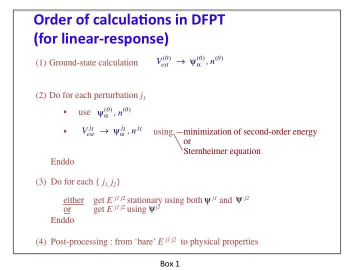
The step 1 is done in a preliminary ground-state calculation (either by an independent run, or by computing them using an earlier dataset before the DFPT calculation). The parallelisation of this step is examined in a separate tutorial.
The step 2 and step 3 are the time-consuming DFPT steps, to which the present tutorial is dedicated, and for which the implementation of the parallelism will be explained. They generate different files, and in particular, one (or several) DDB file(s). As explained in related tutorials (see e.g. Response-Function 1), several perturbations are usually treated in one dataset (hence the “Do for each perturbation”-loop in step 2 of this Schema). For example, in one dataset, although one considers only one phonon wavevector, all the primitive atomic displacements for this wavevector (as determined by the symmetries) can be treated in turn.
The step 4 refers to MRGDDB and ANADDB post-processing of the DDB generated by steps 2 and 3. These are not time-consuming sections. No parallelism is needed.
1.2. The equations to be considered for the computation of the first-order wavefunctions and potentials (step 2 of box 1), which is the really time-consuming part of any DFPT calculation, are presented in box 2.
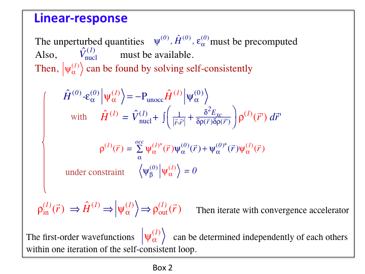
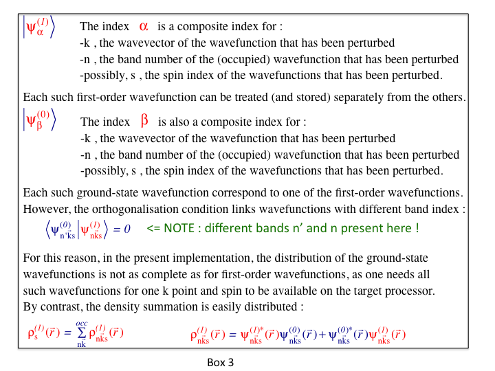
The parallelism currently implemented for the DFPT part of ABINIT is based on the parallel distribution of the most important arrays: the set of first-order and ground-state wavefunctions. While each such wavefunction is stored completely in the memory linked to one computing core (there is no splitting of different parts of one wavefunction between different computing cores - neither in real space nor in reciprocal space), different such wavefunctions might be distributed over different computing cores. This easily achieves a combined k point, spin and band index parallelism, as explained in box 3.
1.3. The parallelism over k points, band index and spin for the set of wavefunctions is implemented in all relevant steps, except for the reading (initialisation) of the ground-state wavefunctions (from an external file). Thus, the most CPU time-consuming parts of the DFPT computations are parallelized. The following are not parallelized:
- input of the set of ground-state wavefunctions
- computing the first-order change of potential from the first-order density, and similar operations that do not depend on the bands or k points.
In the case of small systems, the maximum achievable speed-up will be limited by the input of the set of ground-state wavefunctions. For medium to large systems, the maximum achievable speed-up will be determined by the operations that do not depend on the k point and band indices. Finally, the distribution of the set of ground-state wavefunctions to the computing cores that need them is partly parallelized, as no parallelism over bands can be exploited.
Before continuing you might work in a different subdirectory as for the other tutorials. Why not work_paral_dfpt?
All the input files can be found in the $ABI_TESTS/tutoparal/Input directory. You might have to adapt them to the path of the directory in which you have decided to perform your runs. You can compare your results with reference output files located in $ABI_TESTS/tutoparal/Refs.
In the following, when “(mpirun …) abinit” appears, you have to use a specific command line according to the operating system and architecture of the computer you are using. This can be for instance: mpirun -np 16 abinit
2 Computation of one dynamical matrix (q =0.25 -0.125 0.125) for FCC aluminum
We start by treating the case of a small systems, namely FCC aluminum, for which there is only one atom per unit cell. Of course, many k points are needed, since this is a metal.
2.1. The first step is the pre-computation of the ground state wavefunctions. This is driven by the files tdfpt_01.abi. You should edit it and examine it.
#   FCC Al; 60 special points

#Definition of the unit cell
 acell 3*7.56
 rprim   0 .5 .5  .5 0 .5  .5 .5 0

#Definition of the atom types and pseudopotentials
 ntypat  1
 znucl 13.0
 pp_dirpath "$ABI_PSPDIR"                 # This is the path to the directory were pseudopotentials for tests are stored
 pseudos "Psdj_nc_sr_04_pw_std_psp8/Al.psp8"  # Name and location of the pseudopotential

#Definition of the atoms
 natom  1
 typat  1
 xred  0.0 0.0 0.0

#Numerical parameters of the calculation : planewave basis set and k point grid
 ecut 10
 ngkpt 8 8 8
 nshiftk 4
 shiftk 0.5 0.5 0.5
        0.5 0.0 0.0
        0.0 0.5 0.0
        0.0 0.0 0.5

#Parameters for the SCF procedure
 nstep 20
 occopt 4
 tolvrs 1.0d-18
 nband 5

#Needed for next calculation
 prtden 1

##############################################################
# This section is used only for regression testing of ABINIT #
##############################################################
#%%<BEGIN TEST_INFO>
#%% [setup]
#%% executable = abinit
#%% test_chain = tdfpt_01.abi, tdfpt_02.abi
#%% [files]
#%% [paral_info]
#%% max_nprocs = 4
#%% nprocs_to_test = 4
#%% [NCPU_4]
#%% files_to_test = tdfpt_01_MPI4.abo, tolnlines=  0, tolabs=  0.000e+00, tolrel=  0.000e+00
#%% post_commands =
#%%   ww_mv tdfpt_01_MPI4o_WFK tdfpt_02_MPI4i_WFK;
#%% [extra_info]
#%% authors = X. Gonze
#%% keywords =
#%% description = FCC Al linear response with k point parallelism
#%%<END TEST_INFO>
One relies on a k-point grid of 8x8x8 x 4 shifts (=2048 k points), and 5 bands. The k-point grid sampling is well converged, actually. For this ground-state calculation, symmetries can be used to reduce drastically the number of k points: there are 60 k points in the irreducible Brillouin zone (this cannot be deduced from the examination of the input file, though). In order to treat properly the phonon calculation, the number of bands is larger than the default value, that would have given nband=3. Indeed, several of the unoccupied bands plays a role in the response calculations in the case of metallic occupations. For example, the acoustic sum rule might be largely violated when too few unoccopied bands are treated.
This calculation is very fast, actually. You can launch it:
mpirun -n 4 abinit tdfpt_01.abi > log &
A reference output file is available in $ABI_TESTS/tutoparal/Refs, under the name tdfpt_01.abo. It was obtained using 4 computing cores, and took a few seconds.
2.2. The second step is the DFPT calculation, see the file tdfpt_02.abi
#   FCC Al; ; phonon at 1/4 1/8 1/8

#Definition of DFPT calculation
 rfphon 1
 nqpt   1
 qpt    0.25 -0.125 0.125
 irdwfk 1

#Timing parameters
 prtvol 10
 timopt 1


#Definition of the unit cell
 acell 3*7.56
 rprim   0 .5 .5  .5 0 .5  .5 .5 0

#Definition of the atom types and pseudopotentials
 ntypat  1
 znucl 13.0
 pp_dirpath "$ABI_PSPDIR"                 # This is the path to the directory were pseudopotentials for tests are stored
 pseudos "Psdj_nc_sr_04_pw_std_psp8/Al.psp8"  # Name and location of the pseudopotential

#Definition of the atoms
 natom  1
 typat  1
 xred  0.0 0.0 0.0

#Numerical parameters of the calculation : planewave basis set and k point grid
 ecut 10
 kptopt 3
 ngkpt 8 8 8
 nshiftk 4
 shiftk 0.5 0.5 0.5
        0.5 0.0 0.0
        0.0 0.5 0.0
        0.0 0.0 0.5

#Parameters for the SCF procedure
 nstep 20
 occopt 4
 tolvrs 1.0d-10
 nband 5

##############################################################
# This section is used only for regression testing of ABINIT #
##############################################################
#%%<BEGIN TEST_INFO>
#%% [setup]
#%% executable = abinit
#%% test_chain = tdfpt_01.abi, tdfpt_02.abi
#%% [files]
#%% [paral_info]
#%% max_nprocs = 4
#%% nprocs_to_test = 4
#%% [NCPU_4]
#%% files_to_test = tdfpt_02_MPI4.abo, tolnlines= 15, tolabs=  1.1e-05, tolrel=  1.5e-02
#%% [extra_info]
#%% authors = X. Gonze
#%% keywords =
#%% description = FCC Al linear response with k point parallelism
#%%<END TEST_INFO>
There are three perturbations (three atomic displacements). For the two first perturbations, no symmetry can be used, while for the third, two symmetries can be used to reduce the number of k points to 1024. Hence, for the perfectly scalable sections of the code, the maximum speed up is 5120 (=1024 k points * 5 bands), if you have access to 5120 computing cores. However, the sequential parts of the code dominate at a much, much lower value. Indeed, the sequential parts is actually a few percents of the code on one processor, depending on the machine you run. The speed-up might saturate beyond 8…16 (depending on the machine). Note that the number of processors that you use for this second step is independent of the number of processors that you used for the first step. The only relevant information from the first step is the *_WFK file.
First copy the output of the ground-state calculation so that it can be used as the input of the DFPT calculation:
cp tdfpt_01o_WFK tdfpt_02i_WFK
(A _WFQ file is not needed, as all GS wavefunctions at k+q are present in the GW wavefuction at k). Then, you can launch the calculation:
mpirun -n 4 abinit tdfpt_02.abi > tdfpt_02.log &
A reference output file is given in $ABI_TESTS/tutoparal/Refs, under the name tdfpt_02.abo. Edit it, and examine some information. The calculation has been made with four computing cores:
- mpi_nproc: 4, omp_nthreads: -1 (-1 if OMP is not activated)
The wall clock time is less than 50 seconds :
-
- Proc.   0 individual time (sec): cpu=         28.8  wall=         28.9

================================================================================

 Calculation completed.
.Delivered   0 WARNINGs and   0 COMMENTs to log file.
+Overall time at end (sec) : cpu=        115.4  wall=        115.8
The major result is the phonon frequencies:
  Phonon wavevector (reduced coordinates) :  0.25000 -0.12500  0.12500
 Phonon energies in Hartree :
   6.521506E-04  7.483301E-04  1.099648E-03
 Phonon frequencies in cm-1    :
-  1.431305E+02  1.642395E+02  2.413447E+02
2.3. Because this test case is quite fast, you should play a bit with it. In particular, run it several times, with an increasing number of computing cores (let us say, up to 40 computing cores, at which stage you should have obtained a saturation of the speed-up). You should be able to obtain a decent speedup up to 8 processors, then the gain becomes more and more marginal. Note however that the result is independent (to an exquisite accuracy) of the number of computing cores that is used
Let us explain the timing section. It is present a bit before the end of the output file:
-
- For major independent code sections, cpu and wall times (sec),
-  as well as % of the time and number of calls for node 0-
-<BEGIN_TIMER mpi_nprocs = 4, omp_nthreads = 1, mpi_rank = 0>
- cpu_time =           28.8, wall_time =           28.9
-
- routine                        cpu     %       wall     %      number of calls  Gflops    Speedup Efficacity
-                                                                  (-1=no count)
- fourwf%(pot)                  14.392  12.5     14.443  12.5         170048      -1.00        1.00       1.00
- nonlop(apply)                  2.787   2.4      2.802   2.4         125248      -1.00        0.99       0.99
- nonlop(forces)                 2.609   2.3      2.620   2.3          64000      -1.00        1.00       1.00
- fourwf%(G->r)                  2.044   1.8      2.052   1.8          47124      -1.00        1.00       1.00
- dfpt_vtorho-kpt loop           1.174   1.0      1.177   1.0             21      -1.00        1.00       1.00
- getgh1c_setup                  1.111   1.0      1.114   1.0           8960      -1.00        1.00       1.00
- mkffnl                         1.087   0.9      1.092   0.9          20992      -1.00        1.00       1.00
- projbd                         1.023   0.9      1.036   0.9         286336      -1.00        0.99       0.99
- dfpt_vtowfk(contrib)           0.806   0.7      0.805   0.7             -1      -1.00        1.00       1.00
- others (120)                  -2.787  -2.4     -2.825  -2.4             -1      -1.00        0.99       0.99
-<END_TIMER>
-
- subtotal                      24.246  21.0     24.317  21.0                                  1.00       1.00

- For major independent code sections, cpu and wall times (sec),
- as well as % of the total time and number of calls

-<BEGIN_TIMER mpi_nprocs = 4, omp_nthreads = 1, mpi_rank = world>
- cpu_time =         115.3, wall_time =         115.6
-
- routine                         cpu     %       wall     %      number of calls Gflops    Speedup Efficacity
-                                                                  (-1=no count)
- fourwf%(pot)                  51.717  44.8     51.909  44.9         679543      -1.00        1.00       1.00
- dfpt_vtorho:MPI               12.267  10.6     12.292  10.6             84      -1.00        1.00       1.00
- nonlop(apply)                 10.092   8.8     10.149   8.8         500343      -1.00        0.99       0.99
- nonlop(forces)                 9.520   8.3      9.562   8.3         256000      -1.00        1.00       1.00
- fourwf%(G->r)                  7.367   6.4      7.398   6.4         187320      -1.00        1.00       1.00
- dfpt_vtorho-kpt loop           4.182   3.6      4.193   3.6             84      -1.00        1.00       1.00
- getgh1c_setup                  3.955   3.4      3.967   3.4          35840      -1.00        1.00       1.00
- mkffnl                         3.911   3.4      3.929   3.4          83968      -1.00        1.00       1.00
- projbd                         3.735   3.2      3.780   3.3        1144046      -1.00        0.99       0.99
- dfpt_vtowfk(contrib)           2.754   2.4      2.748   2.4             -4      -1.00        1.00       1.00
- getghc-other                   1.861   1.6      1.790   1.5             -4      -1.00        1.04       1.04
- pspini                         0.861   0.7      0.865   0.7              4      -1.00        0.99       0.99
- newkpt(excl. rwwf   )          0.754   0.7      0.757   0.7             -4      -1.00        1.00       1.00
- others (116)                 -14.132 -12.3    -14.220 -12.3             -1      -1.00        0.99       0.99
-<END_TIMER>

- subtotal                      98.845  85.7     99.120  85.7                                  1.00       1.00
It is made of two groups of data. The first one corresponds to the analysis of the timing for the computing core (node) number 0. The second one is the sum over all computing cores of the data of the first group. Note that there is a factor of four between these two groups, reflecting that the load balance is good.
Let us examine the second group of data in more detail. It corresponds to a decomposition of the most time-consuming parts of the code. Note that the subtotal is 85.7 percent, thus the statistics is not very accurate, as it should be close to 100%. Actually, as of ABINIT v9, there is must be a bug in the timing decomposition, since, e.g. there is a negative time announced for the “others” subroutines.
Anyhow, several of the most time-consuming parts are directly related to application of the Hamiltonian to wavefunctions, namely, fourwf%(pot) (application of the local potential, which implies two Fourier transforms), nonlop(apply) (application of the non-local part of the Hamiltonian), nonlop(forces) (computation of the non-local part of the interatomic forces), fourwf%(G->r) (fourier transform needed to build the first-order density). Also, quite noticeable is dfpt_vtorho:MPI , synchronisation of the MPI parallelism.
A study of the speed-up brought by the k-point parallelism for this simple test case gives the following behaviour, between 1 and 40 cores:
At 8 processors, one gets a speed-up of 7.17, which is quite decent (about 90% efficiency), but 16 processors, the speed-up is only 11.1 (about 70% efficiency), and the efficiency is below 50% at 40 processors, for a speed-up of 19.7 ..
3 Computation of one perturbation for a slab of 29 atoms of barium titanate
3.1. This test, with 29 atoms, is slower, but highlights other aspects of the DFPT parallelism than the Al FCC case. It consists in the computation of one perturbation at qpt 0.0 0.25 0.0 for a 29 atom slab of barium titanate, artificially terminated by a double TiO2 layer on each face, with a reasonable k-point sampling of the Brillouin zone.
The symmetry of the system and perturbation will allow to decrease this sampling to one quarter of the Brillouin zone. E.g. with the k-point sampling ngkpt 4 4 1, there will be actually 4 k-points in the irreducible Brillouin zone for the Ground state calculations. For the DFPT case, only one (binary) symmetry will survive, so that, after the calculation of the frozen-wavefunction part (for which no symmetry is used), the self-consistent part will be done with 8 k points in the corresponding irreducible Brillouin zone. Beyond 8 cores, the parallelisation will be done also on the bands. This will prove to be much more dependent on the computer architecture than the (low-communication) parallelism over k-points.
With the sampling 8 8 1, there will be 32 k points in the irreducible Brillouin zone for the DFPT case. This will allow potentially to use efficiently a larger number of processors, provided the computer architecture and network is good enough.
There are 116 occupied bands. For the ground state calculation, 4 additional conduction bands will be explicitly treated, which will allow better SCF stability thanks to iprcel 45. Note that the value of ecut that is used in the present tutorial is too low to obtain physical results (it should be around 40 Hartree). Also, only one atomic displacement is considered, so that the phonon frequencies delivered at the end of the run are meaningless.
As in the previous case, a preparatory ground-state calculation is needed. We use the input variable autoparal=1 . It does not delivers the best repartition of processors among np_spkpt, npband and npfft, but achieves a decent repartition, usually within a factor of two. With 24 processors, it selects np_spkpt=4 (optimal), npband=3 and npfft=2, while npband=6 and npband=1 would do better. For information, the speeup going from 24 cores to 64 cores is 1.76, not quite the increase of number of processor (2.76). Anyhow, the topics of the tutorial is not the GS calculation.
The input files are provided, in the directory $ABI_TESTS/tutoparal/Input. The preparatory step is driven by tdfpt_03.abi. The real (=DFPT) test case is driven by tdfpt_04.abi. The reference output files are present in $ABI_TESTS/tutoparal/Refs: tdfpt_03_MPI24.abo and tdfpt_04_MPI24.abo. The naming convention is such that the number of cores used to run them is added after the name of the test: the tdfpt_03.abi files are run with 24 cores. The preparatory step takes about 3 minutes, and the DFPT step takes about 3 minutes as well.
#SLAB ending TiO2 double layer
# N=9
# paralelectric configuration

#Parameters that govern parallelism
paral_kgb 1
autoparal 1  # This attempts to find a good distribution of processors. Actually, it is not optimal, but decent.

#Definition of the unit cell
acell 4.0 4.0 28.0 Angstrom

#Definition of the atom types and pseudopotentials
ntypat 3
znucl 56 22 8
pp_dirpath "$ABI_PSPDIR/Psdj_nc_sr_04_pw_std_psp8"
pseudos "Ba.psp8, Ti.psp8, O.psp8"

#Definition of the atoms
natom 29
typat 3 3 2 3 3 2 1 3 3 3 2 1 3 3 3 2 1 3 3 3 2 1 3 3 3 2 3 3 2
            xcart      0.0000000000E+00  0.0000000000E+00 -4.2633349730E+00
                       3.7794522658E+00  3.7794522658E+00 -3.2803418097E+00
                       0.0000000000E+00  3.7794522658E+00 -3.6627278067E+00
                       3.7794522658E+00  0.0000000000E+00  6.5250113947E-01
                       0.0000000000E+00  3.7794522658E+00 -1.0555036964E-01
                       3.7794522658E+00  3.7794522658E+00  3.2682166278E-01
                       0.0000000000E+00  0.0000000000E+00  3.9815918094E+00
                       3.7794522658E+00  3.7794522658E+00  4.0167907030E+00
                       3.7794522658E+00  0.0000000000E+00  7.7541444349E+00
                       0.0000000000E+00  3.7794522658E+00  7.6664087705E+00
                       3.7794522658E+00  3.7794522658E+00  7.7182324796E+00
                       0.0000000000E+00  0.0000000000E+00  1.1412913350E+01
                       3.7794522658E+00  3.7794522658E+00  1.1416615533E+01
                       3.7794522658E+00  0.0000000000E+00  1.5117809063E+01
                       0.0000000000E+00  3.7794522658E+00  1.5117809063E+01
                       3.7794522658E+00  3.7794522658E+00  1.5117809063E+01
                       0.0000000000E+00  0.0000000000E+00  1.8822704777E+01
                       3.7794522658E+00  3.7794522658E+00  1.8819002593E+01
                       3.7794522658E+00  0.0000000000E+00  2.2481473692E+01
                       0.0000000000E+00  3.7794522658E+00  2.2569209355E+01
                       3.7794522658E+00  3.7794522658E+00  2.2517385647E+01
                       0.0000000000E+00  0.0000000000E+00  2.6254026317E+01
                       3.7794522658E+00  3.7794522658E+00  2.6218827423E+01
                       3.7794522658E+00  0.0000000000E+00  2.9583116986E+01
                       0.0000000000E+00  3.7794522658E+00  3.0341168496E+01
                       3.7794522658E+00  3.7794522658E+00  2.9908796464E+01
                       0.0000000000E+00  0.0000000000E+00  3.4498953099E+01
                       3.7794522658E+00  3.7794522658E+00  3.3515959935E+01
                       0.0000000000E+00  3.7794522658E+00  3.3898345933E+01
chksymtnons 0  # The position of the system is such that some symmetry operations have a non-symmorphic shift which
               # is not a simple fraction. This is not a problem for ABINIT, but this input variable must be activated.

#Numerical parameters of the calculation : planewave basis set and k point grid
ecut 15.0
ngkpt 4 4 1
kptopt 1

#Parameters for the SCF procedure
nstep 30
tolvrs 1.0d-18 # This value is much too small for production run (but was chosen to make this tutorial more portable accross platforms).
               # A value 1.0d-12 is more reasonable.
iprcel 45   # This is to help the SCF procedure, work quite well in this case of a slab.

#Electronic structure
nband 120

#%%<BEGIN TEST_INFO>
#%% [setup]
#%% executable = abinit
#%% test_chain = tdfpt_03.abi, tdfpt_04.abi
#%% [files]
#%% [paral_info]
#%% max_nprocs = 24
#%% nprocs_to_test = 24
#%% [NCPU_24]
#%% files_to_test = tdfpt_03_MPI24.abo, tolnlines = 10, tolabs = 5.0e-10, tolrel= 3.0e-3
#%% post_commands =
#%%   ww_mv tdfpt_03_MPI24o_WFK tdfpt_04_MPI24i_WFK
#%% [extra_info]
#%% keywords = NC
#%% description = BaTiO3 linear response calculation
#%%<END TEST_INFO>
#SLAB ending TiO2 double layer
# N=9
# paralelectric configuration

#Parameters for DFPT
rfphon 1
irdwfk 1
rfatpol 1 1
rfdir 0 0 1
nqpt 1
qpt 0.0 0.25  0.0
#prtwf 0

timopt -2
kptopt 3
tolwfr 1.0d-18
tolrde 0.0 # This is a development input variable, used in the present case to avoid load unbalance
           # when studying the scaling with respect to the number of cores. Do not define it in
           # your production runs

#Definition of the unit cell
acell 4.0 4.0 28.0 Angstrom

#Definition of the atom types and pseudopotentials
ntypat 3
znucl 56 22 8
pp_dirpath "$ABI_PSPDIR/Psdj_nc_sr_04_pw_std_psp8"
pseudos "Ba.psp8, Ti.psp8, O.psp8"

#Definition of the atoms
natom 29
typat 3 3 2 3 3 2 1 3 3 3 2 1 3 3 3 2 1 3 3 3 2 1 3 3 3 2 3 3 2
            xcart      0.0000000000E+00  0.0000000000E+00 -4.2633349730E+00
                       3.7794522658E+00  3.7794522658E+00 -3.2803418097E+00
                       0.0000000000E+00  3.7794522658E+00 -3.6627278067E+00
                       3.7794522658E+00  0.0000000000E+00  6.5250113947E-01
                       0.0000000000E+00  3.7794522658E+00 -1.0555036964E-01
                       3.7794522658E+00  3.7794522658E+00  3.2682166278E-01
                       0.0000000000E+00  0.0000000000E+00  3.9815918094E+00
                       3.7794522658E+00  3.7794522658E+00  4.0167907030E+00
                       3.7794522658E+00  0.0000000000E+00  7.7541444349E+00
                       0.0000000000E+00  3.7794522658E+00  7.6664087705E+00
                       3.7794522658E+00  3.7794522658E+00  7.7182324796E+00
                       0.0000000000E+00  0.0000000000E+00  1.1412913350E+01
                       3.7794522658E+00  3.7794522658E+00  1.1416615533E+01
                       3.7794522658E+00  0.0000000000E+00  1.5117809063E+01
                       0.0000000000E+00  3.7794522658E+00  1.5117809063E+01
                       3.7794522658E+00  3.7794522658E+00  1.5117809063E+01
                       0.0000000000E+00  0.0000000000E+00  1.8822704777E+01
                       3.7794522658E+00  3.7794522658E+00  1.8819002593E+01
                       3.7794522658E+00  0.0000000000E+00  2.2481473692E+01
                       0.0000000000E+00  3.7794522658E+00  2.2569209355E+01
                       3.7794522658E+00  3.7794522658E+00  2.2517385647E+01
                       0.0000000000E+00  0.0000000000E+00  2.6254026317E+01
                       3.7794522658E+00  3.7794522658E+00  2.6218827423E+01
                       3.7794522658E+00  0.0000000000E+00  2.9583116986E+01
                       0.0000000000E+00  3.7794522658E+00  3.0341168496E+01
                       3.7794522658E+00  3.7794522658E+00  2.9908796464E+01
                       0.0000000000E+00  0.0000000000E+00  3.4498953099E+01
                       3.7794522658E+00  3.7794522658E+00  3.3515959935E+01
                       0.0000000000E+00  3.7794522658E+00  3.3898345933E+01
chksymtnons 0

#Numerical parameters of the calculation : planewave basis set and k point grid
ecut 15.0
ngkpt 4 4 1

#Parameters for the SCF procedure
nstep 30

#Electronic structure
nband 116    # Only the occupied states - will ease the convergence
#prtden 0

#%%<BEGIN TEST_INFO>
#%% [setup]
#%% executable = abinit
#%% test_chain = tdfpt_03.abi, tdfpt_04.abi
#%% [files]
#%% [paral_info]
#%% max_nprocs = 24
#%% nprocs_to_test = 24
#%% [NCPU_24]
#%% files_to_test = tdfpt_04_MPI24.abo, tolnlines = 12, tolabs = 1e-07, tolrel= 0.01
#%% post_commands =
#%%   ww_mv tdfpt_03_MPI24o_WFK tdfpt_04_MPI24i_WFK
#%% [extra_info]
#%% keywords = NC
#%% description = BaTiO3 linear response calculation
#%%<END TEST_INFO>
You can run now these test cases. For tdfpt_03, with autoparal=1, you will be able to run on different numbers of processors compatible with nkpt=4, nband=120 and ngfft=[30 30 192], detected by ABINIT. Alternatively, you might decide to explicitly define np_spkpt, npband and npfft. At variance, for tdfpt_04, no adaptation of the input file is needed to be able to run on an arbitrary number of processors. To launch the ground-state computation, type:
mpirun -n 24 abinit tdfpt_03.abi > log &
then copy the output of the ground-state calculation so that it can be used as the input of the DFPT calculation:
mv tdfpt_03o_WFK tdfpt_04i_WFK
and launch the calculation:
mpirun -n 24 abinit tdfpt_04.abi > log &
Now, examine the obtained output file for test 04, especially the timing.
In the reference file $ABI_TESTS/tutoparal/Refs/tdfpt_04_MPI24.abo, with 24 computing cores, the timing section delivers:
- For major independent code sections, cpu and wall times (sec),
-  as well as % of the time and number of calls for node 0-
-<BEGIN_TIMER mpi_nprocs = 24, omp_nthreads = 1, mpi_rank = 0>
- cpu_time =          159.9, wall_time =          160.0
-
- routine                        cpu     %       wall     %      number of calls  Gflops    Speedup Efficacity
-                                                                  (-1=no count)
- projbd                        46.305   1.2     46.345   1.2          11520      -1.00        1.00       1.00
- nonlop(apply)                 42.180   1.1     42.183   1.1           5760      -1.00        1.00       1.00
- dfpt_vtorho:MPI               25.087   0.7     25.085   0.7             30      -1.00        1.00       1.00
- fourwf%(pot)                  22.435   0.6     22.436   0.6           6930      -1.00        1.00       1.00
- nonlop(forces)                 5.485   0.1      5.486   0.1           4563      -1.00        1.00       1.00
- fourwf%(G->r)                  4.445   0.1      4.446   0.1           2340      -1.00        1.00       1.00
- pspini                         2.311   0.1      2.311   0.1              1      -1.00        1.00       1.00

<...>

- For major independent code sections, cpu and wall times (sec),
- as well as % of the total time and number of calls

-<BEGIN_TIMER mpi_nprocs = 24, omp_nthreads = 1, mpi_rank = world>
- cpu_time =        3826.4, wall_time =        3828.0
-
- routine                         cpu     %       wall     %      number of calls Gflops    Speedup Efficacity
-                                                                  (-1=no count)
- projbd                      1238.539  32.4   1239.573  32.4         278400      -1.00        1.00       1.00
- nonlop(apply)               1012.783  26.5   1012.982  26.5         139200      -1.00        1.00       1.00
- fourwf%(pot)                 544.047  14.2    544.201  14.2         167040      -1.00        1.00       1.00
- dfpt_vtorho:MPI              450.196  11.8    450.170  11.8            720      -1.00        1.00       1.00
- nonlop(forces)               131.081   3.4    131.129   3.4         108576      -1.00        1.00       1.00
- fourwf%(G->r)                107.885   2.8    107.930   2.8          55680      -1.00        1.00       1.00
- pspini                        54.945   1.4     54.943   1.4             24      -1.00        1.00       1.00

<...>

- others (99)                  -98.669  -2.6    -99.848  -2.6             -1      -1.00        0.99       0.99
-<END_TIMER>

- subtotal                    3569.873  93.3   3570.325  93.3                                  1.00       1.00
You will notice that the run took about 160 seconds (wall clock time).. The sum of the major independent code sections is reasonably close to 100%. You might now explore the behaviour of the CPU time for different numbers of compute cores (consider values below and above 24 processors). Some time-consuming routines will benefit from the parallelism, some other will not.
The kpoint + band parallelism will efficiently work for many important sections of the code: projbd, fourwf%(pot), nonlop(apply), fourwf%(G->r). In this test, the product nkpt (the effective number of k points for the current perturbation) times nband is 8*120=960. Of course, the total speed-up will saturate well below this value, as there are some non-parallelized sections of the code.
In the above-mentioned list, the kpoint+band parallelism cannot be exploited (or is badly exploited) in several sections of the code : “dfpt_vtorho:MPI”, about 12 percents of the total time of the run on 24 processors, “pspini”, about 1.4 percent. This amounts to about ⅛ of the total. However, the scalability of the band parallelisation is rather poor, and effective saturation in this case already happens at 16 processor.
A study of the speed-up brought by the combined k-point and band parallelism for this test case on a 2 AMD EPYC 7502 machine (2 CPUS, each with 32 cores) gives the following behaviour, between 1 and 40 cores:
The additional band parallelism is very efficient when running with 16 cores, bringing 14.77 speed-up, while using only the k point parallelism, with 6 cores, gives 7.67 speed-up. However, the behaviour is disappointing beyond 16 cores, or even for a number of processors which is not a multiple of 8.
Such a behaviour might be different on your machine.
3.2. A better parallelism can be seen if the number of k-points is brought back to a converged value (8x8x1). Again, Try this if you have more than 100 processors at hand.
Set in your input files tdfpt_03.abi and tdfpt_04.abo :
ngkpt 8 8 1 ! This should replace ngkpt 4 4 1
and launch again the preliminary step, then the DFPT step. Then, you can practice the DFPT calculation by varying the number of computing cores. For the latter, you could even consider varying the number of self-consistent iterations to see the initialisation effects (small value of nstep), or target a value giving converged results (nstep 50 instead of nstep 18). The energy cut-off might also be increased (e.g. ecut 40 Hartree gives a much better value). Indeed, with a large value of k points, and large value of nstep, you might be able to obtain a speed-up of more than one hundred for the DFPT calculation, when compared to a sequential run (see below). Keep track of the time for each computing core number, to observe the scaling.
On a machine with a good communication network, the following results were observed in 2011. The Wall clock timing decreases from
- Proc. 0 individual time (sec): cpu= 2977.3 wall= 2977.3
with 16 processors to
- Proc. 0 individual time (sec): cpu= 513.2 wall= 513.2
with 128 processors.
The next figure presents the speed-up of a typical calculation with increasing number of computing cores (also, the efficiency of the calculation).
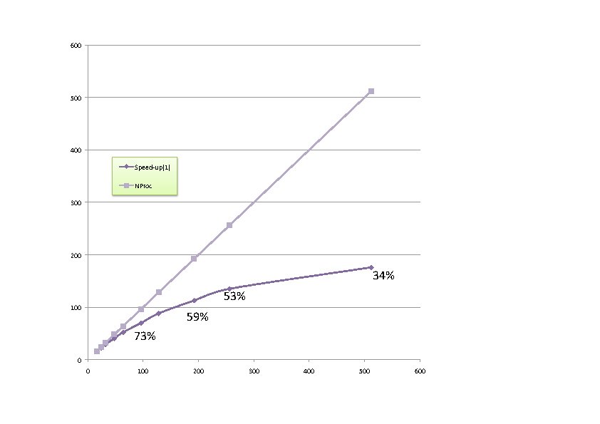
Beyond 300 computing cores, the sequential parts of the code start to dominate. With more realistic computing parameters (ecut 40), they dominate only beyond 600 processors.
However, on the same (recent, but with slow connection beyond 32 cores) computer than for the ngkpt 4 4 1 case, the saturation sets in already beyond 16 cores, with the following behaviour (the reference is taken with respect to the timing at 4 processors):
Thus, it is very important that you gain some understanding of the scaling of your typical runs for your particular computer, and that you know the parameters (especially nkpt) of your calculations. Up to 4 or 8 cores, the ABINIT scaling will usually be very good, if k-point parallelism is possible. In the range between 10 and 100 cores, the speed-up might still be good, but this will depend on details.
This last example is the end of the present tutorial. The basics of the current implementation of the parallelism for the DFPT part of ABINIT have been explained, then you have explored two test cases: one for a small cell materials, with lots of k points, and another one, medium-size, in which the k point and band parallelism must be used. It might reveal efficient, but this will depend on the detail of your calculation and your computer architecture.