Phonon-limited mobility

This tutorial discusses how to compute phonon-limited carrier mobilities in semiconductors within the self-energy relaxation time approximation (SERTA) and the momentum relaxation time approximation (MRTA), taking the specific case of AlAs as an example.

It is assumed the user has already completed the two tutorials RF1 and RF2, and that he/she is familiar with the calculation of ground state and response properties, in particular phonons, Born effective charges and dielectric tensor. The user should have read the introduction tutorial for the EPH code before running these examples.

This lesson should take about 1.5 hour.

Formalism

Before starting, it is worth summarizing the most important equations implemented in the code. For a more detailed description of the ABINIT implementation, please consult [Brunin2020b].

Our goal is to find an approximated solution to the linearized Boltzmann transport equation (BTE) [Ashcroft1976] within the SERTA/MRTA approximation [Giustino2017]. SERTA/MRTA are more accurate than the constant relaxation time approximation (CRTA) as the microscopic e-ph scattering mechanism is now included thus leading to carrier lifetimes $\tau$ that depend on the band index $n$ and the wavevector $\kk$. Keep in mind, however, that both SERTA and MRTA are still a approximated solutions to the BTE and that a more rigorous approach would require to solve the BTE iteratively and/or the inclusion of many-body effects at different levels. For a review of the different possible approaches see the review paper [Ponce2020].

In the SERTA, the transport linewidth is given by the imaginary part of the electron-phonon (e-ph) self-energy evaluated at the KS energy [Giustino2017]. The linewidth of the electron state $n\kk$ due to the scattering with phonons is given by

$$\begin{equation} \begin{split} \lim_{\eta \rightarrow 0^+} & \Im\{\Sigma^\FM_{n\kk}(\enk)\} = \pi \sum_{m,\nu} \int_\BZ \frac{d\qq}{\Omega_\BZ} |\gkkp|^2\\ & \times \left[ (n_\qnu + f_{m\kk+\qq}) \delta(\enk - \emkq + \wqnu) \right.\\ & \left. + (n_\qnu + 1 - f_{m\kk+\qq}) \delta(\enk - \emkq - \wqnu ) \right] \end{split} \label{eq:imagfanks_selfen} \end{equation}$$

where $\nu$ is the phonon mode, $m$ the final electron state (after the scattering), $n_\qnu(T)$ is the Bose-Einstein occupation number, $f_{m\kk+\qq}(T, \ef)$ is the Fermi-Dirac occupation function, $\enk$ is the energy of the electron state, and $\wqnu$ is the phonon frequency for the phonon wavevector $\qq$. The integration is performed over the BZ for the phonon wavectors and $\gkkp$ is the e-ph matrix element. Only the Fan-Migdal (FM) part contributes to the linewidth as the Debye-Waller term is Hermitian.

In the SERTA, the transport lifetime $\tau_{n\mathbf{k}}$ is inversely proportional to the e-ph self-energy linewidth:

$$\begin{align} \frac{1}{\tau_{n\kk}} = 2 \lim_{\eta \rightarrow 0^+} \Im\{\Sigma^\FM_{n\kk}(\enk)\}. \label{eq:fanlifetime} \end{align}$$

In the MRTA, the back-scattering is included by expressing the transport lifetime as:

$$\begin{equation} \begin{split} \frac{1}{\tau_{n\kk}} & = 2 \pi \sum_{m,\nu} \int_\BZ \frac{d\qq}{\Omega_\BZ} |\gkkp|^2 \left( 1 - \frac{\vnk \cdot \vmkq}{|\vnk|^2} \right) \\ & \times \left[ (n_\qnu + f_{m\kk+\qq}) \delta(\enk - \emkq + \wqnu) \right.\\ & \left. + (n_\qnu + 1 - f_{m\kk+\qq}) \delta(\enk - \emkq - \wqnu ) \right]. \end{split} \label{eq:mrta} \end{equation}$$

where $\vnka$ is the $\alpha$-th Cartesian component of the velocity operator

$$\vnk = \PDER{\enk}{\kk} = \langle \nk | \dfrac{\partial{H}}{\partial{\kk}} | \nk \rangle.$$

that can be computed with DFPT.

Important

Note that the present formalism does not take into account contributions to the transport lifetime given by other scattering processes such as defects, ionized impurities in doped semiconductors, e-e interaction, grain boundary scattering etc. These effects may be relevant depending on the system and/or the temperature under investigation but they are not treated in this tutorial as here we are mainly focusing on room temperature and non-degenerate semiconductors, conditions in which e-ph scattering is one of the most important contributions.

Last but not least, we are assuming that carriers can be described by Bloch states with a well-defined excitation energy (band picture). Polaronic effects such as those discussed in this tutorial are not captured by the present approach.

The generalized transport coefficients are defined by:

$$\begin{equation} \mcL^{(m)}_{\alpha\beta} = - \sum_n \int \frac{d\kk}{\Omega_\BZ} \vnka \vnkb\, \tau_{n\kk} (\enk-\ef)^m \left.\frac{\partial f}{\partial\varepsilon}\right|_{\enk} \label{eq:transport_lc} \end{equation}$$

These quantities can be used to obtain different transport tensors such as the electrical conductivity $\sigma$, Peltier ($\Pi$) and Seebeck coefficient (S), and charge carrier contribution to the thermal conductivity tensors [Madsen2018]. The electrical conductivity tensor, for instance, is given by

$$\begin{equation} \sigma_{\alpha\beta} = \frac{1}{\Omega} \mcL_{\alpha\beta}^{(0)} \label{eq:transport_sigma} \end{equation}$$

and can be divided into hole and electron contributions

$$\begin{equation} \sigma = n_e \mu_{e} + n_h \mu_{h} \label{eq:mobility} \end{equation}$$

where $n_e$ and $n_h$ are the electron and hole concentrations in the conduction and valence bands respectively, and $\mu_e$ and $\mu_h$ are the electron and hole mobilities, which can be obtained by selecting the conduction or valences states $n$ in Eq. \eqref{eq:transport_lc}.

For electrons, we have

$$\begin{equation} \begin{split} n_e = \sum_{n\in \text{CB}} \int \dfrac{d\kk}{\Omega_\BZ} f_{n\kk}, \\ \mu_e = \dfrac{1}{n_e \Omega}\, \mcL_{n\in \text{CB}}^{(0)} \end{split} \end{equation}$$

where $n\in\text{CB}$ denotes states in the conduction bands. Similar expressions hold for holes. At zero total carrier concentration, the Fermi level $\ef$ is located inside the band gap so that $n_e = n_h$.

A typical computation of mobilities requires different steps that are summarized in the introduction page for the EPH code. Here we only describe the e-ph related part, i.e the blue-box in the workflow presented in the previous page. For this purpose, we use eph_task -4 to compute only the imaginary part of the SE at the KS energy and explain other important aspects related to this kind of calculation.

All the results of the calculation are saved in netcdf format in the SIGPEPH.nc file, while the main output file is used to output selected quantities, mainly for testing purposes. Post-processing and visualisation tools are provided by AbiPy. See e.g. the README of AbiPy and the AbiPy tutorials.

Note

Supposing you made your own installation of ABINIT, the input files to run the examples are in the ~abinit/tests/ directory where ~abinit is the absolute path of the abinit top-level directory. If you have NOT made your own install, ask your system administrator where to find the package, especially the executable and test files.

In case you work on your own PC or workstation, to make things easier, we suggest you define some handy environment variables by executing the following lines in the terminal:

export ABI_HOME=Replace_with_absolute_path_to_abinit_top_level_dir # Change this line
export PATH=$ABI_HOME/src/98_main/:$PATH      # Do not change this line: path to executable
export ABI_TESTS=$ABI_HOME/tests/             # Do not change this line: path to tests dir
export ABI_PSPDIR=$ABI_TESTS/Psps_for_tests/  # Do not change this line: path to pseudos dir

Examples in this tutorial use these shell variables: copy and paste the code snippets into the terminal (remember to set ABI_HOME first!) or, alternatively, source the set_abienv.sh script located in the ~abinit directory:

source ~abinit/set_abienv.sh

The ‘export PATH’ line adds the directory containing the executables to your PATH so that you can invoke the code by simply typing abinit in the terminal instead of providing the absolute path.

To execute the tutorials, create a working directory (Work*) and copy there the input files of the lesson.

Most of the tutorials do not rely on parallelism (except specific tutorials on parallelism). However you can run most of the tutorial examples in parallel with MPI, see the topic on parallelism.

Ground state and phonons of fcc AlAs

Before beginning, you might consider creating a different subdirectory to work in. Why not create Work_eph4mob ?

The file teph4mob_1.abi is the input file for the first step (GS + DFPT perturbations for all the $\qq$-points in the IBZ). Copy it to the working directory with:

cd $ABI_TUTORESPFN/Input
mkdir Work_eph4mob
cd Work_eph4mob
cp ../teph4mob_1.abi .

View tests/tutorespfn/Input/teph4mob_1.abi

This step might be quite time-consuming so you may want to immediately start the job in background with:

abinit teph4mob_1.abi > teph4mob_1.log 2> err &

The calculation is done for AlAs, the same crystalline material as in the first two DFPT tutorials. For further details about this first step, please refer to the first and second tutorials on DFPT.

Important

Since AlAs is a polar semiconductor, we need to compute with DFPT the Born effective charges $\bm{Z}^*$ as well and the static dielectric tensor $\bm{\ee}^\infty$. These quantities are then used to treat the long-range (LR) part of the dynamical matrix in the Fourier interpolation of the phonon frequencies as well as in the Fourier interpolation of the DFPT potentials, as discussed in the EPH introduction.

Merging the derivative databases and potentials

Once the DFPT calculation is completed, use the mrgddb tool to merge the eight partial DDB files corresponding to datasets 3-10 of teph4mob_1. These partial DDB files contain the dynamical matrices for the 8 $\qq$-points in the IBZ, as well as the dielectric tensor and the Born effective charges. Name the new DDB file teph4mob_2_DDB.

File $ABI_TUTORESPFN/Input/teph4mob_2.abi is an example of input file for mrgddb.

View tests/tutorespfn/Input/teph4mob_2.abi

Copy the file in the Work_eph4mob directory, and run mrgddb using:

mrgddb < teph4mob_2.abi

Tip

Alternatively, one can specify the name of the output DDB and the list of input DDB files to be merged directly via the command line. This approach is quite handy especially if used in conjuction with shell globbing and the “star” syntax:

mrgddb teph4mob_2_DDB teph4mob_1o_DS*_DDB

Use mrgddb –help to access the documentation.

Now use the mrgdv tool to merge the 29 DFPT POT files corresponding to datasets 3-10 of teph4mob_1. Name the new file teph4mob_3_DVDB.

File $ABI_TUTORESPFN/Input/teph4mob_3.abi is an example of input file for mrgdv.

View tests/tutorespfn/Input/teph4mob_3.abi

You can copy it in the Work_eph4mob directory, and then merge the files with:

mrgdv < teph4mob_3.abi

Tip

Alternatively, one can use the command line.

mrgdv merge teph4mob_3_DVDB teph4mob_1o_DS*_POT*

Use mrgdv –help to access the documentation.

We now have all the phonon-related files needed to compute the mobility. The DDB will be used to Fourier interpolate the phonon frequencies on an arbitrarily dense $\qq$-mesh while the DVDB will be used to Fourier interpolate the DFPT scattering potentials [Brunin2020b]. The only ingredient that is still missing is the WFK file with the GS wavefunctions on the dense $\kk$-mesh.

Warning

In real computations, you should always compute the electronic band structure along a $\kk$-path to have a qualitative understanding of the band dispersion, the position of the band edges, and the value of the band gap(s). Note also that there are several parts of the EPH code in which it is assumed that no vibrational instability is present so you should always look at the phonon spectrum computed by the code. Do not expect to obtain meaningful results if purely imaginary phonon frequencies (a.k.a negative frequencies) are present.

Calculation of the dense WFK file

Converging transport properties requires careful convergence tests both for $\kk$-points and $\qq$-points. A dense $\qq$-mesh is needed to obtain high-quality lifetimes, whereas a dense $\kk$-sampling is needed to have a good sampling of the electron (hole) pockets. All these studies are explained later and left as an additional excercise. In this tutorial, indeed, we need to find some compromise between accuracy and computational cost hence a single $\kk$-mesh is used in all our examples.

The computation of the dense WFK file is similar to a NSCF band structure computation. The main difference is that we need wavefunctions on a $\kk$-mesh instead of a $\kk$-path because these wavevectors are needed to evaluate integrals in the BZ. The file $ABI_TUTORESPFN/Input/teph4mob_4.abi is an example of such computation.

View tests/tutorespfn/Input/teph4mob_4.abi

It consists of two parts:

1. the first one (dataset 1) computes the GS wavefunctions,
2. the second one (datasets 2-3) computes the dense WFK that will be used to compute mobilities. We also compute another (denser) WFK file that will be used with the double-grid method explained later. As we are mainly interested in electron mobilities (conduction bands) we need to include enough empty bands in the NSCF WFK computation (nband = 8).

Copy the file in the Work_eph4mob directory, and run ABINIT:

abinit teph4mob_4.abi > teph4mob_4.log 2> err &

Important

In the last part of the tutorial, we explain how to avoid the NSCF computation for all the $\kk$-points in the IBZ and produce a partial WFK file containing only the wavevectors relevant for transport properties. This trick is crucial to reach dense meshes but can also be used for coarser meshes if you want to accelerate the NSCF part and reduced the size of the WFK file.

Calculation of the mobility

We begin by explaining how to specify the basic input variables required for a standard mobility calculation. The file $ABI_TUTORESPFN/Input/teph4mob_5.abi is an example of such computation.

View tests/tutorespfn/Input/teph4mob_5.abi

First of all, we need to read the WFK, the DDB and the DVDB files produced previously. Since it is not possible to run mobility calculations with a single input file and datasets, we use strings to specify the path of the input files:

getwfk_filepath "teph4mob_4o_DS2_WFK"
getddb_filepath "teph4mob_2_DDB"
getdvdb_filepath "teph4mob_3_DVDB"

Now copy the input file in the Work_eph4mob directory, and run the code with:

abinit teph4mob_5.abi > teph4mob_5.log 2> err &

The job should take $\sim$15 seconds on a recent CPU.

We now discuss the meaning of the e-ph variables in more detail:

• optdriver 7 activates the EPH driver

• eph_task -4 tells ABINIT that we only need the imaginary part of the e-ph self-energy at the KS energy.

• The homogeneous $\kk$-mesh corresponding to the WFK file is specified by ngkpt 24 24 24. The code aborts with an error if ngkpt is not the same as the one found in the input WFK file. At present, multiple shifts (nshiftk > 1) are not supported.

• ddb_ngqpt defines the initial $\qq$-grid used for the DFPT computation (4×4×4 in this example)

• eph_ngqpt_fine defines the dense $\qq$-mesh where the scattering potentials are interpolated and the e-ph matrix elements are computed.

  Warning

  ngkpt and eph_ngqpt_fine should be commensurate. More specifically, ngkpt must be a multiple of the $\qq$-mesh (eph_ngqpt_fine) because the WFK should contain all the $\kk$- and $\kq$-points. In most cases, ngkpt == eph_ngqpt_fine. It is however possible to use fewer $\qq$-points. Note also that ngkpt does not necessarily correspond to the $\kk$-mesh used for the computation of transport quantities, see the following discussion.

• We work within the rigid band approximation and introduce a small electron doping: eph_doping = -1e+15 that corresponds to 1e+15 electrons per cm$^3$. To obtain results that are representative of the intrinsic mobility, we suggest to use a very small value, for instance $10^{15}$ to $10^{18}$ electrons per cm$^3$. Alternatively, one can specify the doping via eph_extrael or eph_fermie. We also set occopt to 3 to correctly compute the location of the Fermi level using the Fermi-Dirac occupation function as we are dealing with the physical temperature and not a fictitious broadening for numerical integration purposes.

• The list of physical temperatures is specified by tmesh.

  Note

  The computational cost increases with the number of temperatures although not necessarily in a linear fashion. For the initial convergence studies, we suggest to start from a relatively small number of temperatures covering the range of interest. The T-mesh can be densified aftwerwards while keeping the same T-range once converged parameters are found.

  Note that transport properties at low temperatures are more difficult to converge as the derivative of the Fermi-Dirac distribution is strongly peaked around the Fermi level hence a very dense sampling is needed to converge the BZ integrals. In a nutshell, avoid low temperatures unless you are really interested in this regime.

• By default, the code use the tetrahedron method [Bloechl1994] to perform the integration in $\qq$-mesh. This allows to efficiently filter out the $\qq$-points that do not contribute to the lifetimes since these transitions are not compatible with energy and crystalline-momentum conservation. The use of the tetrahedron method is automatically activated when eph_task is set to -4. It is possible to change this behaviour by using eph_intmeth albeit not recommended as the calculation will become significantly slower. If using the Gaussian method, one must converge the self-energy with respect to zcut (or eph_fsmear if eph_task is set to 1), By default, zcut is set to a very large value.

• The sigma_erange variable defines the energy window, below the VBM and above the CBM, where the lifetimes will be computed. Since the mobility integrals involve the derivative of the Fermi-Dirac occupation function centered on the Fermi level, it is possible to restrict the computation to those $\kk$-points that contribute to the mobility integral. The value of the derivative, indeed, decreases rapidly as we go further from the Fermi level hence only the states close to the band edges contribute. This variable should be subject to a convergence study as explained in the next section.

• boxcutmin and mixprec are used to accelerate the computation, see the introductory tutorial.

We now examine the log file in detail. After the standard output of the input variables, the code reports the different parameters used for the treatment of the long-range part of the DFPT potentials: the Born effective charges, the high-frequency dielectric constant and the dynamical quadrupole tensor. Make sure to have all of them in order to obtain an accurate interpolation of the scattering potentials, see discussion in [Brunin2020].

Important

At present (November 05, 2024 ), the inclusion of the dynamical quadrupoles in the EPH code is not available in the public version so you should have the following in the log file:

Have dielectric tensor: yes
Have Born effective charges: yes
Have quadrupoles: no
Have electric field: no

The code then outputs different quantities. For instance, ABINIT finds the list of $\kk$-points belonging to the dense mesh that are located within the energy window (sigma_erange):

Found 3 k-points within erange:  0.000  0.150  (eV)

Over the initial 413 $\kk$-points in the IBZ, only 3 will be computed!

The value of the Fermi level (a.k.a electronic chemical potential $\mu_e(T)$) as a function of T is computed and printed afterwards. Make sure that $\mu_e$ is far enough from the band edges so that the computed mobility can be considered as intrinsic: the values of D_v and D_c should be large compared to ~3 kT else you enter the degenerate regime or the highly-degenerate case (when the Fermi level is inside the bands) and additional physical phenomena start to play a role.

 Position of CBM/VBM with respect to the Fermi level:
 Notations: mu_e = Fermi level, D_v = (mu_e - VBM), D_c = (CBM - mu_e)

  T(K)   kT (eV)  mu_e (eV)  D_v (eV)   D_c (eV)
   5.0     0.000     3.521     1.165     0.004
  64.0     0.006     3.475     1.118     0.051
 123.0     0.011     3.428     1.071     0.098
 182.0     0.016     3.379     1.023     0.146
 241.0     0.021     3.328     0.972     0.197
 300.0     0.026     3.274     0.918     0.251

ABINIT then reads the WFK file and interpolates the scattering potentials to obtain the e-ph matrix elements. The use of the tetrahedron method allows to significantly reduce the $\qq$-points:

qpoints_oracle: calculation of tau_nk will need: 15 q-points in the IBZ. (nqibz_eff / nqibz):   3.6 [%]

Once this is done, the code starts looping over the 3 $\kk$-points for which the lifetimes are needed.

Computing self-energy matrix elements for k-point: [ 4.5833E-01,  4.5833E-01,  0.0000E+00] [ 1 / 3 ]

You can find various information for each $\kk$-point, such as:

• the total number of $\qq$-points in the irreducible zone defined by the little group of $\kk$ (called IBZ(k) in the code),

• the number of $\qq$-point in the $\text{IBZ}_k$ contributing to the imaginary part of $\Sigma_\nk$ (in most cases, this number will be much smaller than the total number of $\qq$-points in the $\text{IBZ}_k$)

• the wall-time each step takes.

Finally, we have the results for the lifetimes (TAU) in the teph4mob_5.abo file:

K-point: [ 4.5833E-01,  4.5833E-01,  0.0000E+00], T:    5.0 [K], mu_e:    3.521
   B    eKS    SE2(eKS)  TAU(eKS)  DeKS
   5   3.573    0.000  36639.9    0.000

View tests/tutorespfn/Refs/teph4mob_5.abo

Tip

As already mentioned in the introduction, all the results are stored in the SIGEPH.nc file. With AbiPy , one can easily access to all the data of the computation. For instance, one can plot the electron linewidths as a function of the KS energy using the abiopen.py script:

abiopen.py teph4mob_5o_SIGEPH.nc --expose

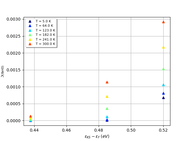
Well, the figure is not so impressive but this is normal as we are computing only 3 $\kk$-wavevectors still there are some points that are worth discussing. Note how the linewidths at the CBM are very small at low temperature. For the CBM, indeed, only phonon absorption is allowed and there are few vibrational states populated at low T. The linewidth at the CBM increses with T since high energy phonon states starts to be populated and more scattering channels become available.

At the end of the main output file, the diagonal elements of the SERTA/MRTA mobility tensor $\sigma_{ij}$ are reported for the three Cartesian directions and all temperatures.

 Cartesian component of SERTA mobility tensor: xx
 Temperature [K]             e/h density [cm^-3]          e/h mobility [cm^2/Vs]
            5.00        0.10E+16        0.00E+00            0.00            0.00
           64.00        0.10E+16        0.00E+00           40.76            0.00
          123.00        0.10E+16        0.00E+00          356.24            0.00
          182.00        0.10E+16        0.00E+00          435.51            0.00
          241.00        0.10E+16        0.00E+00          433.89            0.00
          300.00        0.10E+16        0.25E+05          379.06            0.00

 Cartesian component of MRTA mobility tensor: xx
 Temperature [K]             e/h density [cm^-3]          e/h mobility [cm^2/Vs]
            5.00        0.10E+16        0.00E+00            0.00            0.00
           64.00        0.10E+16        0.00E+00           39.67            0.00
          123.00        0.10E+16        0.00E+00          374.94            0.00
          182.00        0.10E+16        0.00E+00          470.73            0.00
          241.00        0.10E+16        0.00E+00          469.55            0.00
          300.00        0.10E+16        0.25E+05          411.23            0.00

The temperature is first given then the electron (e) and hole (h) densities followed by the corresponding (SERTA/MRTA) mobilities. In our input file, we considered only electrons and this explains why the values for holes are zero. In this particular case, the difference between SERTA and MRTA is not very large but the two approximation may give significantly different results in other systems. According to recent works the MRTA results are expected to be closer to ones obtained by iteratively solving the BTE.

Tip

You can also run the transport driver in standalone mode by setting eph_task 7, provided you already have the lifetimes in an external SIGEPH.nc file specified via getsigeph_filepath. This task is relatively fast even in serial execution although some parts (in particular the computation of DOS-like quantities) can benefit from MPI.

Now that we know how to obtain the mobility in a semiconductor for given $\kk$- and $\qq$-meshes, we can give additional details about convergence studies and discuss extra tricks to significantly decrease the computational cost.

Convergence w.r.t. the energy range

The first convergence study consists in determining the energy range around the band edge to be used for the computation of $\tau_{n\kk}$. We can do that by performing mobility computations with fixed $\kk$- and $\qq$-meshes and increasing values of sigma_erange.

Tip

The code can compute both electron and hole mobilities in a single run but this is not the recommended procedure as the $\qq$-point filtering is expected to be less efficient. Moreover electrons and holes may require a different $\kk$-sampling to convergence depending on the dispersion of the bands. As a consequence, we suggest to compute electrons and holes with different input files.

The file $$ABI_TUTORESPFN/Input/teph4mob_6.abi is an example of such computation.

View tests/tutorespfn/Input/teph4mob_6.abi

Copy the input file in the Work_eph4mob directory, and run ABINIT:

abinit teph4mob_6.abi > teph4mob_6.log 2> err &

This run should take a few minutes.

We can now analyze the variation of the mobility with respect to sigma_erange.

TODO: Add script to analyze convergence wrt sigma_erange

This study shows that an energy window of ~0.15 above the CBM is enough to converge so we use this value in the subsequent calculations.

Warning

One should perform this convergence study with a $\kk$-mesh that is already dense enough to capture the band dispersion correctly. In this case, we are using a 24×24×24 mesh, which is not very dense for such computations. This means that, when increasing sigma_erange, no additional $\kk$-point is included as the sampling is too coarse. This is the case for the first three datasets (3 $\kk$-points), and the last two datasets (6 $\kk$-points). If a finer mesh was used, the number of $\kk$-points would have increased in a more monotonic way. For instance, in Silicon, a 45×45×45 $\kk$-mesh could be used to determine sigma_erange.

Convergence w.r.t. the k/q meshes

Once the energy window is set, we can start to converge the mobility with respect to the dense $\kk$- and $\qq$-meshes. The previous computations used 24×24×24 $\kk$- and $\qq$-meshes. This is quite far from convergence. Just to give you an idea, silicon requires a 45×45×45 $\kk$-mesh and 90×90×90 $\qq$-mesh to reach convergence within 5%.

Tip

As a rule of thumb, a $\qq$-mesh twice as dense in each direction as the $\kk$-mesh, is needed to obtain accurate values for the linewidth and achieve fast convergence of the integrals in $\kk$-space [Brunin2020b]. Possible exceptions are systems with very small effective masses (e.g. GaAs) in which a very dense $\kk$-sampling is needed to sample the electron (hole) pockets. In this case, using the same sampling for electrons and phonons may be enough to converge.

To compute the mobility with a $\qq$-mesh twice as dense as the $\kk$-mesh, there are two possible approaches:

1. Run a computation with:

   • ngkpt 90 90 90 (nshiftk 1 and shiftk 0 0 0)
   • eph_ngqpt_fine 90 90 90,
   • sigma_ngkpt 45 45 45.

   using sigma_ngkpt to select the $\kk$-points in $\Sigma_\nk$ belonging to the 45×45×45 mesh, but now each lifetime is computed with a 90×90×90 $\qq$-mesh.

2. Run a computation with:

   • ngkpt 90 90 90, (nshiftk 1 and shiftk 0 0 0)
   • eph_ngqpt_fine 90 90 90,
   • sigma_ngkpt 90 90 90.

   Following this approach, we compute lifetimes on a 90×90×90 $\kk$- and the integration is perfomed on the same $\qq$-mesh. You can then run again the transport driver only, by setting eph_task 7 and transport_ngkpt 45 45 45 to downsample the $\kk$-mesh used to integrate the mobility in $\kk$-space. This second option has the advantage that it delivers two mobilities in one-shot but it would be overkilling if a 45×45×45/90×90×90 k/q sampling is already enough.

You can run again the previous input files by densifying the different meshes. For the densest grids, you might need to run with multiple MPI processes. You should obtain something like this for $T$ = 300 K:

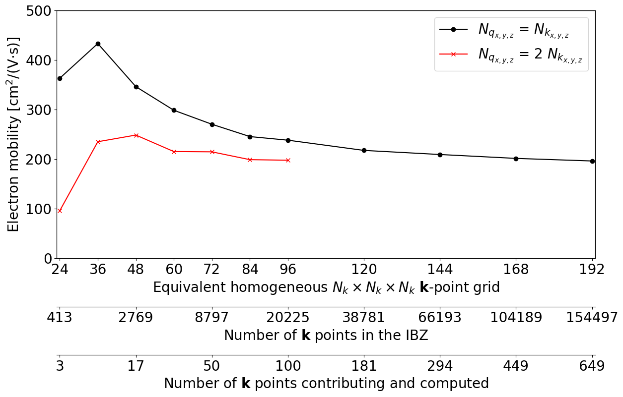
Sorry for repeating it again but, the inputs of this tutorial have been tuned to make the computations quite fast, but the final results are far from convergence. In order to get sensible results, one should use a denser DFPT $\qq$-mesh (around 9×9×9), and a larger cutoff energy ecut. Obviously, these parameters depend on the system under investigation.

Double-grid technique

Another possibility to improve the results without increasing the computation time significantly is the double-grid (DG) technique [Brunin2020b]. In this method, a coarse sampling is used for the $\kk$- and the $\qq$-mesh for the e-ph matrix elements, but a finer mesh is used to interpolate the weights for the delta functions associated to phonon absorption/emission. This technique allows one to accelerate the convergence while keeping the computational cost and the memory requirements at a reasonable level.

Important

The efficiency of the DG approach depends on the strength of the polar Frohlich divergence: if the divergence is difficult to integrate numerically, the coarse $\qq$-mesh for the e-ph matrix elements will have to be densified.

The DG technique requires a second WFK file, containing the KS eigenvalues on the fine mesh. You can specify the path to the fine WFK file using getwfkfine_filepath as in:

getwfkfine_filepath "teph4mob_4o_DS3_WFK"

The file $$ABI_TUTORESPFN/Input/teph4mob_7.abi (first dataset) is an example of such computation.

View tests/tutorespfn/Input/teph4mob_7.abi

Copy the input file in the Work_eph4mob directory, and run ABINIT:

abinit teph4mob_7.abi > teph4mob_7.log 2> err &

In the log file, you will now find information about the double-grid method:

coarse:                24          24          24
fine:                  48          48          48

The SERTA mobility obtained at 300 K is 163.84 cm$^2$/V/s. Using a 48×48×48 $\qq$-mesh for the matrix elements as well would give 96.97 (using sigma_ngkpt 24 24 24). The result is indeed improved, since using a 24×24×24 mesh both for electrons and phonons gives 379.06. You can also use a finer mesh, but always multiple of the initial coarse mesh (in this case, 72×72×72, 96×96×96, etc). It is worth noticing that, according to our tests, there is very little use to go beyond a mesh three times as dense as the coarse one. Using a 72×72×72 fine mesh for the energies gives a mobility of 152.30 cm$^2$/V/s, and a 96×96×96 mesh leads to 149.38 cm$^2$/V/s: the improvement is indeed rather limited.

Important

As a rule of thumb, consider to use the DG method for systems in which the tetrahedron filter is not able to reduce the number of $\qq$-points in the integrals below 5% for a significant fraction of the $\kk$-points in the sigma_erange energy window. This may happen if there are multiple equivalent pockets and thus many intra-valley scattering channels. In this case, the computation of $\tau_\nk$ may require several minutes (2-10) per $\kk$-point and calculations performed with the same $\kk$- and $\qq$-mesh start to be expensive when the BZ sampling gets denser.

In-place restart

All the results of the calculation are stored in a single SIGEPH.nc file for all the $\kk$-points (and spins) considered. The list of $\kk$-points is initialized at the beginning of the calculation and an internal table in the netcdf file stores the status of each $\kk$-point (whether it has been computed or not). This means that calculations that are killed by the resource manager due to time limit can reuse the SIGEPH file to perform an automatic in-place restart. Just set eph_restart to 1 in the input file and rerun the job

Important

There is no harm in setting eph_restart to 1 from the begining but keep in mind that the code will restart the calculation from scratch if all the $\kk$-points in the SIGEPH.nc have been computed (a backup copy is kept). So we do not recommended the use of this option in MultiDataset mode. Again, MultiDataset are evil when it comes to high-performance!

Transport calculation from SIGEPH.nc

The routine that computes carrier mobilites is automatically invoked when eph_task -4 is used and a RTA.nc file with the final results is produced. There are however cases in which one would like to compute mobilities starting from a pre-existent SIGEPH.nc without performing a full calculation from scratch. In this case, use eph_task 7 and specify the name of the SIGEPH.nc file with getsigeph_filepath. The advanced input variable transport_ngkpt can be used to downsample the $\kk$-mesh used in the mobility integrals.

MPI parallelism and memory requirements

There are five different MPI levels that can be used to distribute the workload and the most memory-demanding data structures. By default, the code tries to reach some compromise between memory requirements and time to solution by activating the parallelism over perturbations and then the $\qq$-point parallelism if no input is provided by the user. You can however specify manually the MPI distribution across the five different levels by using eph_np_pqbks (a list of 5 integers). The product of these five numbers must be equal to the total number of MPI processes.

The first entry defines the number of processes for the parallelization over perturbations. The allowed value range between 1 and 3 × natom, and should be a divisor of 3 × natom to distribute the work equally. The higher this number, the lower the memory requirements at the price of increased MPI communication. The second entry determines the parallelization over the $\qq$-points in the IBZ. This parallelization level allows one to decrease both the computational time as well as memory although it’s not always possible to distribute the load equally among the processes. The parallelization over bands is usually not relevant for mobility computations as only a few states close to the VBM or CBM are usually included. The MPI parallelism over $\kk$-points and spins is very efficient but it requires HDF5 with MPI-IO support and, besides, memory won’t scale. Use these additional two levels if the memory requirements are under control and you want to boost the calculation.

How to reduce the memory requirements

As mentioned above, the memory will scale with the number of MPI processors used for the $\qq$-point and the perturbation communicators. However, there might be tricky systems in which you start to experience memory shortage that prevents you from running with many MPI processes. This problem should show up for very dense $\kk$/$\qq$ meshes. As a rule of thumb, mobility calculations with meshes denser than e.g 200x200x200 start to be very memory demanding and the execution will slow down because several algorithms and internal tables for the BZ sampling and the tetrahedron method start to dominate. The double grid technique helps mitigate this bottleneck. In some cases, you may try to reduce slightly the value of sigma_erange to reduce the memory requirements.

Note also that the EPH code allocates a relatively small buffer to store the Bloch states involved in transport calculations but unfortunately the $\kk$-points are not easy to distribute with MPI. Moreover the size of this array depends on the electronic dispersion: systems with several relatively flat bands around the band edges require more memory. To reduce the memory for the wavefunctions, the code uses internal buffers in single precision. This option is enabled at configure time by using enable_gw_dpc="no" (this is the default behaviour).

If these tricks do not solve your problem, consider using OpenMP threads. The code is not highly-optimized for OpenMP but a couple of threads may be useful to avoid replicating memory at the MPI level. As a rule of thumb, 2-4 OpenMP threads should be OK provided you link with threaded FFT and BLAS libraries. To compile ABINIT with OpenMP support and link with a threaded library see the corresponding section in the ABINIT_build tutorial.

Warning

Last but not least, do not use datasets: split the calculation into different input files and optimize the number of MPI processes according to the dimension of the problem. You have been warned!

How to compute the WFK only for k-points close to the band edges

As we have already seen in the previous sections, a relatively small number of $\kk$-points close to the band edges is usually sufficient to converge mobilities. Yet, in the NSCF run, we computed a WFK file for all the $\kk$-points in the IBZ hence we spent a lot of resources to compute and store states that are not needed for phonon-limited mobilities.

In principle, it is possible to restrict the NSCF calculation to the relevant $\kk$-points provided we have a cheap and good-enough method to predict whether the wavevector is inside the energy window without solving the KS eigevalue problem exactly. For example, one can use the star-function interpolation by Shankland-Koelling-Wood (SKW) [Shankland1971], [Koelling1986], [Madsen2006], [Madsen2018] which requires as input a set of eigenvalues in the IBZ and a single parameter defining the basis set for the interpolation.

There are several technical problems that should be addressed at the level of the internal implementation but the idea is relatively simple and goes as follows:

1. Compute the KS eigenvalues on a relatively coarse $\kk$-mesh in the IBZ
2. Use this coarse WFK file to interpolate the eigenvalues on a much denser $\kk$-mesh specified by the user.
3. Find the wavevectors of the dense mesh inside an energy window specified by the user and store the list of $\kk$-points in a external file (KERANGE.nc).
4. Use this external file to run a NSCF calculation only for these $\kk$-points. At the end of the NSCF job, ABINIT will produce a customized WFK file on the dense mesh that can be used to run calculations for phonon-limited mobilities

An example will help clarify.

Suppose we have computed a WFK file with a NSCF run using a 16x16x16 $\kk$-mesh (let’s call it 161616_WFK) and we want to compute mobilites with the much denser 64x64x64 $\kk$-mesh. In this case, use

• optdriver = 8
• wfk_task = “wfk_kpts_erange”

to read the WFK file specified by getwfk_filepath, find the wavevectors belonging to the sigma_ngkpt $\kk$-mesh inside the energy window defined by sigma_erange and produce a KERANGE.nc file. The parameters defining the SKW interpolation are specified by einterp.

A typical input file for this step looks like:

optdriver 8
wfk_task "wfk_kpts_erange"
getwfk_filepath "161616_WFK"

# Define fine k-mesh for the interpolation
sigma_ngkpt   64 64 64
sigma_nshiftk 1
sigma_shiftk  0 0 0

sigma_erange 0.0 0.2 eV   # Select kpts in fine mesh within this energy window.
einterp 1 5 0 0           # Parameters for star-function interpolation

This input produces a KERANGE.nc file (let’s call it out_KERANGE) that can be used via the getkerange_filepath variable as a starting point to perfom a NSCF run with the following variables:

getkerange_filepath "out_KERANGE.nc"
getden_filepath "161616_DEN"    # Read DEN file to initialize NSCF run
getwfk_filepath "161616_WFK"    # Init GS wavefunctions from this file (optional)
iscf  -2
tolwfr 1e-18
kptopt 0                        # Important!

# These variables must be consistent with the values of
# sigma_ngkpt, sigma_shiftk used in the previous step
ngkpt    64 64 64
nshiftk  1
shiftk   0.0 0.0 0.0

This part will produce a customized Fortran WFK file with ngkpt = 64 64 64 in which only the states listed in the KERANGE.nc netcdf file have been computed. This WKF file can then be used in the EPH code to compute mobilites. For further examples see v9[57], and v9[61].

Note that the two tests cannot be executed in multidataset mode with a single input file. Also, keep in mind that the quality of the interpolation depends on the initial coarse $\kk$-mesh so we recommended to look at the interpolant, see discussion at the end of the introductory tutorial.

Important

It is also a good idea to use an energy window that is larger than the one that will be employed to compute the mobility in the EPH code. As a rule of thumb, increase sigma_erange by 0.15 eV when computing the KERANGE.nc file. This should be however tested in each case.