First tutorial on GW

The quasi-particle band structure of Silicon in the GW approximation.

This tutorial aims at showing how to calculate self-energy corrections to the DFT Kohn-Sham (KS) eigenvalues in the GW approximation.

A brief description of the formalism and of the equations implemented in the code can be found in the GW_notes. The different formulas of the GW formalism have been written in a pdf document by Valerio Olevano who also wrote the first version of this tutorial. For a much more consistent discussion of the theoretical aspects of the GW method we refer the reader to the review article Quasiparticle calculations in solids by W.G Aulbur et al also available here.

It is suggested to acknowledge the efforts of developers of the GW part of ABINIT, by citing the 2005 ABINIT publication.

The user should be familiarized with the four basic tutorials of ABINIT, see the tutorial home page. After this first tutorial on GW, you should read the second GW tutorial.

This tutorial should take about 2 hours.

Note

Supposing you made your own installation of ABINIT, the input files to run the examples are in the ~abinit/tests/ directory where ~abinit is the absolute path of the abinit top-level directory. If you have NOT made your own install, ask your system administrator where to find the package, especially the executable and test files.

In case you work on your own PC or workstation, to make things easier, we suggest you define some handy environment variables by executing the following lines in the terminal:

export ABI_HOME=Replace_with_absolute_path_to_abinit_top_level_dir # Change this line
export PATH=$ABI_HOME/src/98_main/:$PATH      # Do not change this line: path to executable
export ABI_TESTS=$ABI_HOME/tests/             # Do not change this line: path to tests dir
export ABI_PSPDIR=$ABI_TESTS/Pspdir/  # Do not change this line: path to pseudos dir

Examples in this tutorial use these shell variables: copy and paste the code snippets into the terminal (remember to set ABI_HOME first!) or, alternatively, source the set_abienv.sh script located in the ~abinit directory:

source ~abinit/set_abienv.sh

The ‘export PATH’ line adds the directory containing the executables to your PATH so that you can invoke the code by simply typing abinit in the terminal instead of providing the absolute path.

To execute the tutorials, create a working directory (Work*) and copy there the input files of the lesson.

Most of the tutorials do not rely on parallelism (except specific tutorials on parallelism). However you can run most of the tutorial examples in parallel with MPI, see the topic on parallelism.

1 General example of an almost converged GW calculation

Before beginning, you might consider to work in a different subdirectory as for the other tutorials. Why not Work_gw1?

At the end of tutorial 3, we computed the KS band structure of silicon. In this approximation, the band dispersion as well as the band widths are reasonable but the band gaps are qualitatively wrong. Now we will compute the band gaps much more accurately, using the so-called GW approximation.

We start by an example, in which we show how to perform in a single input file the calculation of the ground state density, the Kohn Sham band structure, the screening, and the GW corrections. We use reasonable values for the parameters of the calculation. The discussion on the convergence tests is postponed to the next paragraphs. We will see that GW calculations are much more time-consuming than the computation of the KS eigenvalues.

So, let us run immediately this calculation, and while it is running, we will explain what has been done.

mkdir Work_gw1
cd Work_gw1
cp $ABI_TESTS/tutorial/Input/tgw1_1.abi .

Then, issue:

    abinit tgw1_1.abi > log 2> err &

Please run this job in background because it takes about 1 minute. In the meantime, you should read the following.

1.a The four steps of a GW calculation.

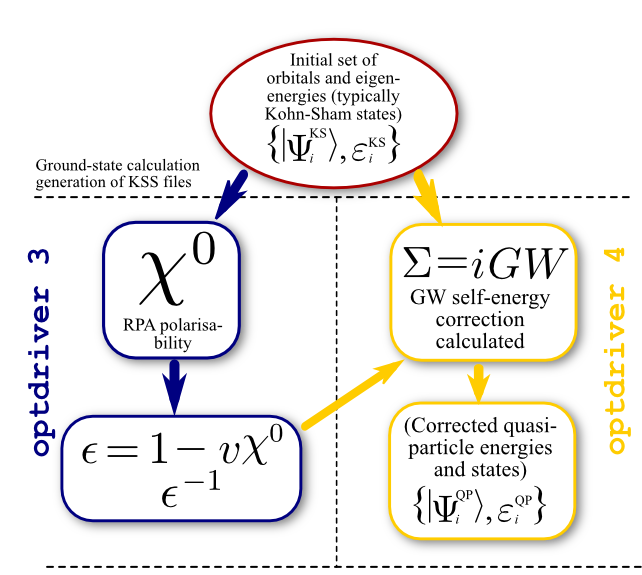
In order to perform a standard one-shot GW calculation one has to:

1. Run a converged Ground State calculation to obtain the self-consistent density.

2. Perform a non self-consistent run to compute the KS eigenvalues and the eigenfunctions including several empty states. Note that, unlike standard band structure calculations, here the KS states must be computed on a regular grid of k-points. (This limitation is also present with hybrid functional calculations).

3. Use optdriver = 3 to compute the independent-particle susceptibility \(\chi^0\) on a regular grid of q-points, for at least two frequencies (usually, \(\omega=0\) and a purely imaginary frequency - of the order of the plasmon frequency, a dozen of eV). The inverse dielectric matrix \(\epsilon^{-1}\) is then obtained via matrix inversion and stored in an external file (SCR). The list of q-points is automatically defined by the k-mesh used to generate the KS states in the previous step.

4. Use optdriver = 4 to compute the self-energy \(\Sigma\) matrix elements for a given set of k-points in order to obtain the GW quasiparticle energies. Note that the k-point must belong to the k-mesh used to generate the WFK file in step 2.

The flowchart diagram of a standard one-shot run is depicted in the figure below.

The input file tgw1_1.abi has precisely that structure: there are four datasets.

The first dataset performs the SCF calculation to get the density. The second dataset reads the previous density file and performs a NSCF run including several empty states. The third dataset reads the WFK file produced in the previous step and drives the computation of susceptibility and dielectric matrices, producing another specialized file, tgw1_xo_DS2_SCR (_SCR for “Screening”, actually the inverse dielectric matrix \(\epsilon^{-1}\)). Then, in the fourth dataset, the code calculates the quasiparticle energies for the 4^th and 5^th bands at the \(\Gamma\) point.

So, you can edit this tgw1_1.abi file.

View tests/tutorial/Input/tgw1_1.abi

In the first half of the file, you will find specialized input variables for the datasets 1 to 4.

In the second half of the file, one find the dataset-independent information, namely, input variables describing the cell, atom types, number, position, planewave cut-off energy, SCF convergence parameters driving the KS band structure calculation.

1.b Generating the Kohn-Sham band structure: the WFK file.

Dataset 1 drives a rather standard SCF calculation. It is worth noticing that we use tolvrs to stop the SCF cycle because we want a well-converged KS potential to be used in the subsequent NSCF calculation. Dataset 2 computes 100 bands and we set nbdbuf to 20 so that only the first 80 states must be converged within tolwfr. The 20 highest energy states are simply not considered when checking the convergence.

    ###########
    # Dataset 1
    ############
    # SCF-GS run
    nband1  6
    tolvrs1 1.0e-10

    ############
    # Dataset 2
    ############
    # Definition of parameters for the calculation of the WFK file
    nband2     100       # Number of (occ and empty) bands to be computed
    nbdbuf2     20       # Do not apply the convergence criterium to the last 20 bands (faster)
    iscf2       -2
    getden2     -1
    tolwfr2  1.0d-12     # Will stop when this tolerance is achieved

Important

The nbdbuf trick allows us to save several minimization steps because the last bands usually require more iterations to converge in the iterative diagonalization algorithms. Also note that it is a very good idea to increase significantly the value of nbdbuf when computing many empty states. As a rule of thumb, use 10% of nband or even more in complicated systems. This can really make a huge difference at the level of the wall time.

1.c Generating the screening: the SCR file.

In dataset 3, the calculation of the screening (KS susceptibility \(\chi^0\) and then inverse dielectric matrix \(\epsilon^{-1}\)) is performed. We need to set optdriver=3 to do that:

    optdriver3  3        # Screening calculation

The getwfk input variable is similar to other “get” input variables of ABINIT:

    getwfk3     -1       # Obtain WFK file from previous dataset

In this case, it tells the code to use the WFK file calculated in the previous dataset.

Then, three input variables describe the computation:

    nband3      60   # Bands used in the screening calculation
    ecuteps3    3.6  # Cut-off energy of the planewave set to represent the dielectric matrix

In this case, we use 60 bands to calculate the KS response function \(\chi^{0}\). The dimension of \(\chi^{0}\), as well as all the other matrices (\(\chi\), \(\epsilon^{-1}\)) is determined by the cut-off energy ecuteps = 3.6 Hartree, which yields 169 planewaves in our case.

Finally, we define the frequencies at which the screening must be evaluated: \(\omega=0.0\) eV and the imaginary frequency \(\omega= i 16.7\) eV. The latter is determined by the input variable ppmfrq

    ppmfrq3    16.7 eV  # Imaginary frequency where to calculate the screening

The two frequencies are used to calculate the plasmon-pole model parameters. For the non-zero frequency, it is recommended to use a value close to the plasmon frequency for the plasmon-pole model to work well. Plasmons frequencies are usually close to 0.5 Hartree. The parameters for the screening calculation are not far from the ones that give converged Electron Energy Loss Function (\(-\mathrm{Im} \epsilon^{-1}_{00}\)) spectra, so that one can start up by using indications from EELS calculations existing in literature. Alternatively, ABINIT can compute an approximate plasmon frequency using the Drude formula. This is activated by letting ppmfrq to its default value. It is actually safer to use the Drude value than to use blindly a value like 16.7 eV for other materials than silicon.

1.d Computing the GW energies.

In dataset 4 the calculation of the Self-Energy matrix elements is performed. One needs to define the driver option as well as the _WFK and _SCR files.

    optdriver4  4       # Self-Energy calculation
    getwfk4    -2       # Obtain WFK file from dataset 2
    getscr4    -1       # Obtain SCR file from previous dataset

The getscr input variable is similar to other “get” input variables of ABINIT.

Then, comes the definition of parameters needed to compute the self-energy. As for the computation of the susceptibility and dielectric matrices, one must define the set of bands and two sets of planewaves:

    nband4       80      # Bands to be used in the Self-Energy calculation
    ecutsigx4   8.0      # Dimension of the G sum in Sigma_x
                         # (the dimension in Sigma_c is controlled by npweps)

In this case, nband controls the number of bands used to calculate the correlation part of the Self-Energy while ecutsigx gives the number of planewaves used to calculate \(\Sigma_x\) (the exchange part of the self-energy). The size of the planewave set used to compute \(\Sigma_c\) (the correlation part of the self-energy) is controlled by ecuteps and cannot be larger than the value used to generate the SCR file. For the initial convergence studies, it is advised to set ecutsigx to a value as high as ecut since, anyway, this parameter is not much influential on the total computational time. Note that the exact treatment of the exchange part requires, in principle, ecutsigx = 4 * ecut.

Then, come the parameters defining the k-points and the band indices for which the quasiparticle energies will be computed:

    nkptgw4      1           # number of k-point where to calculate the GW correction
    kptgw4  0.00  0.00  0.00 # k-points
    bdgw4       4  5         # calculate GW corrections for bands from 4 to 5

nkptgw defines the number of k-points for which the GW corrections will be computed. The k-point reduced coordinates are specified in kptgw while bdgw gives the minimum/maximum band whose energies are calculated for each selected k-point.

Important

These k-points must belong to the k-mesh used to generate the WFK file. Hence if you wish the GW correction in a particular k-point, you should choose a grid containing it. Usually this is done by taking the k-point grid where the convergence is achieved and shifting it such as at least one k-point is placed on the wished position in the Brillouin zone.

There is an additional parameter, called zcut, (not studied here) related to the self-energy computation. It is meant to avoid some divergences that might occur in the calculation due to integrable poles along the integration path.

1.e Examination of the output file.

Your calculation should have ended now. Let’s examine the output file. Open tgw1_1.abo in your preferred editor and find the section corresponding to DATASET 3.

View tests/tutorial/Refs/tgw1_1.abo

After the description of the unit cell and of the pseudopotentials, you will find the list of k-points used for the electrons and the grid of q-points (in the Irreducible part of the Brillouin Zone) on which the susceptibility and dielectric matrices will be computed.

 ==== K-mesh for the wavefunctions ====
 Number of points in the irreducible wedge :     6
 Reduced coordinates and weights :

     1)    -2.50000000E-01 -2.50000000E-01  0.00000000E+00       0.18750
     2)    -2.50000000E-01  2.50000000E-01  0.00000000E+00       0.37500
     3)     5.00000000E-01  5.00000000E-01  0.00000000E+00       0.09375
     4)    -2.50000000E-01  5.00000000E-01  2.50000000E-01       0.18750
     5)     5.00000000E-01  0.00000000E+00  0.00000000E+00       0.12500
     6)     0.00000000E+00  0.00000000E+00  0.00000000E+00       0.03125

 Together with 48 symmetry operations and time-reversal symmetry
 yields    32 points in the full Brillouin Zone.


 ==== Q-mesh for the screening function ====
 Number of points in the irreducible wedge :     6
 Reduced coordinates and weights :

     1)     0.00000000E+00  0.00000000E+00  0.00000000E+00       0.03125
     2)     5.00000000E-01  5.00000000E-01  0.00000000E+00       0.09375
     3)     5.00000000E-01  2.50000000E-01  2.50000000E-01       0.37500
     4)     0.00000000E+00  5.00000000E-01  0.00000000E+00       0.12500
     5)     5.00000000E-01 -2.50000000E-01  2.50000000E-01       0.18750
     6)     0.00000000E+00 -2.50000000E-01 -2.50000000E-01       0.18750

 Together with 48 symmetry operations and time-reversal symmetry
 yields    32 points in the full Brillouin Zone.

The q-mesh is the set of all the possible momentum transfers. These points are obtained as all the possible differences among the k-points ( \(\mathbf{q} =\mathbf{k}-\mathbf{k}'\) ) of the grid chosen to generate the WFK file. From the last statement it is clear the importance of choosing homogeneous k-point grids in order to minimize the number of q-points is clear.

After this section, the code prints the parameters of the FFT grid needed to represent the wavefunctions and to compute their convolution (required for the screening matrices). Then we have some information about the MPI distribution of the bands and the total number of valence electrons computed by integrating the density in the unit cell.

 setmesh: FFT mesh size selected  =  20x 20x 20
          total number of points  =     8000


- screening: taking advantage of time-reversal symmetry
- Maximum band index for partially occupied states nbvw = 4
- Remaining bands to be divided among processors   nbcw = 56
- Number of bands treated by each node ~56

With the valence density, one can obtain the classical Drude plasma frequency. The next lines calculate the average density of the system, and evaluate the Wigner radius \(r_s\), then compute the Drude plasma frequency, reported as omega_plasma.

 Number of electrons calculated from density =    7.9999; Expected =    8.0000
 average of density, n =  0.029628
 r_s =    2.0048
 omega_plasma =   16.6039 [eV]

This omega_plasma is the value used when the default for ppmfrq, namely 0.0, is specified. It is in fact the second frequency where the code calculates the dielectric matrix to adjust the plasmon-pole model parameters.

It has been found that Drude plasma frequency is a reasonable value where to adjust the model. The control over this parameter is however left to the user in order to check that the result does not change when changing ppmfrq. One has to be careful with finite systems or with systems having semicore electrons. If the result depends much on ppmfrq, then the plasmon-pole model is not appropriate and one should go beyond it by taking into account a full dynamical dependence in the screening (see later, the contour-deformation method). However, the plasmon-pole model has been found to work well for a very large range of solid-state systems when focusing only on the real part of the GW corrections in the band gap region.

At the end of the screening calculation, the macroscopic dielectric constant is printed:

      dielectric constant =  22.4176
      dielectric constant without local fields =  24.7005

Note

Note that the convergence in the dielectric constant does not guarantee the convergence in the GW corrections and vice-versa. In fact, the dielectric constant is representative of only one element i.e. the head of the full dielectric matrix. Even if the convergence on the dielectric constant with local fields takes somehow into account also other non-diagonal elements. In a GW calculation the whole \(\epsilon^{-1}\) matrix is used to build the Self-Energy operator.

The dielectric constant reported here is the so-called RPA dielectric constant due to the electrons. Although evaluated at zero frequency, it is understood that the ionic response is not included (this term can be computed with DFPT and ANADDB). The RPA dielectric constant restricted to electronic effects is also not the same as the one computed in the DFPT part of ABINIT, that includes exchange-correlation effects.

We now enter the fourth dataset. As for dataset 3, after some general information (origin of WFK file, header, description of unit cell, k-points, q-points), the description of the FFT grid and jellium parameters, there is the echo of parameters for the plasmon-pole model, and the inverse dielectric function (the screening). The self-energy operator has been constructed, and one can evaluate the GW energies for each state.

The final results are:

--- !SelfEnergy_ee
kpoint     : [   0.000,    0.000,    0.000, ]
spin       : 1
KS_gap     :    2.544
QP_gap     :    3.110
Delta_QP_KS:    0.567
data: !SigmaeeData |
     Band     E0 <VxcDFT>   SigX SigC(E0)      Z dSigC/dE  Sig(E)    E-E0       E
        2   4.418 -11.332 -13.262   1.352   0.766  -0.305 -11.775  -0.443   3.975
        3   4.418 -11.332 -13.262   1.352   0.766  -0.305 -11.775  -0.443   3.975
        4   4.418 -11.332 -13.262   1.352   0.766  -0.305 -11.775  -0.443   3.975
        5   6.961 -10.028  -5.550  -4.316   0.766  -0.305  -9.904   0.124   7.085
        6   6.961 -10.028  -5.550  -4.316   0.766  -0.305  -9.904   0.124   7.085
        7   6.961 -10.028  -5.550  -4.316   0.766  -0.305  -9.904   0.124   7.085
...

For the desired k-point (\(\Gamma\) point), for state 4, then state 5, one finds different information in the SigmaeeData section:

• E0 is the KS eigenenergy
• VxcDFT gives the KS exchange-correlation potential expectation value
• SigX gives the exchange contribution to the self-energy
• SigC(E0) gives the correlation contribution to the self-energy, evaluated at the KS eigenenergy
• Z is the renormalisation factor
• dSigC/dE is the energy derivative of SigC with respect to the energy
• SigC(E) gives the correlation contribution to the self-energy, evaluated at the GW energy
• E-E0 is the difference between GW energy and KS eigenenergy
• E is the final GW quasiparticle energy

In this case, prior to the SigmaeeData section, the direct band gap was also analyzed: KS_gap is the direct KS gap at that particular k-point (and spin, in the case of spin-polarized calculations), QP_gap is the GW one, and Delta_QP_KS is the difference. This direct gap is always computed between the band whose number is equal to the number of electrons in the cell divided by two (integer part, in case of spin-polarized calculation), and the next one. This means that the value reported by the code may be wrong if the final QP energies obtained in the perturbative approach are not ordered by increasing energy anymore. So it’s always a good idea to check that the “gap” reported by the code corresponds to the real QP direct gap.

Warning

For a metal, these two bands do not systematically lie below and above the KS Fermi energy - but the concept of a direct gap is not relevant in that case. Moreover one should compute the Fermi energy of the QP system.

It is seen that the KS exchange-correlation potential expectation value for the state 4 (a valence state) is rather close to the exchange self-energy correction. For that state, the correlation correction is small, and the difference between KS and GW energies is also small (0.128 eV). By contrast, the exchange self-energy is much smaller than the average Kohn-Sham potential for the state 5 (a conduction state), but the correlation correction is much larger than for state 4. On the whole, the difference between Kohn-Sham and GW energies is not very large, but nevertheless, it is quite important when compared with the size of the gap.

If AbiPy is installed on your machine, you can use the abiopen.py script with the --print option to extract the results from the SIGRES.nc file and print them to terminal:

abiopen.py tgw1_1o_DS4_SIGRES.nc -p

================================= Structure =================================
Full Formula (Si2)
Reduced Formula: Si
abc   :   3.839136   3.839136   3.839136
angles:  60.000000  60.000000  60.000000
Sites (2)
  #  SP       a     b     c
---  ----  ----  ----  ----
  0  Si    0     0     0
  1  Si    0.25  0.25  0.25

Abinit Spacegroup: spgid: 0, num_spatial_symmetries: 48, has_timerev: True, symmorphic: True

============================== Kohn-Sham bands ==============================
Number of electrons: 8.0, Fermi level: 4.773 (eV)
nsppol: 1, nkpt: 6, mband: 80, nspinor: 1, nspden: 1
smearing scheme: none, tsmear_eV: 0.272, occopt: 1
Direct gap:
    Energy: 2.544 (eV)
    Initial state: spin: 0, kpt: [+0.000, +0.000, +0.000], weight: 0.031, band: 3, eig: 4.418, occ: 2.000
    Final state:   spin: 0, kpt: [+0.000, +0.000, +0.000], weight: 0.031, band: 4, eig: 6.961, occ: 0.000
Fundamental gap:
    Energy: 0.710 (eV)
    Initial state: spin: 0, kpt: [+0.000, +0.000, +0.000], weight: 0.031, band: 3, eig: 4.418, occ: 2.000
    Final state:   spin: 0, kpt: [+0.500, +0.500, +0.000], weight: 0.094, band: 4, eig: 5.128, occ: 0.000
Bandwidth: 11.985 (eV)
Valence maximum located at:
    spin: 0, kpt: [+0.000, +0.000, +0.000], weight: 0.031, band: 3, eig: 4.418, occ: 2.000
Conduction minimum located at:
    spin: 0, kpt: [+0.500, +0.500, +0.000], weight: 0.094, band: 4, eig: 5.128, occ: 0.000

TIP: Call set_fermie_to_vbm() to set the Fermi level to the VBM if this is a non-magnetic semiconductor


=============================== QP direct gaps ===============================
QP_dirgap: 3.110 (eV) for K-point: [+0.000, +0.000, +0.000] $\Gamma$, spin: 0


============== QP results for each k-point and spin (all in eV) ==============
K-point: [+0.000, +0.000, +0.000] $\Gamma$, spin: 0
   band     e0    qpe  qpe_diago   vxcme  sigxme  sigcmee0  vUme    ze0
1     1  4.418  3.975      3.840 -11.332 -13.262     1.352   0.0  0.766
2     2  4.418  3.975      3.840 -11.332 -13.262     1.352   0.0  0.766
3     3  4.418  3.975      3.840 -11.332 -13.262     1.352   0.0  0.766
4     4  6.961  7.085      7.123 -10.028  -5.550    -4.316   0.0  0.766
5     5  6.961  7.085      7.123 -10.028  -5.550    -4.316   0.0  0.766
6     6  6.961  7.085      7.123 -10.028  -5.550    -4.316   0.0  0.766

For further details about the SIGRES.nc file and the AbiPy API see the Sigres notebook .

2 Preparing convergence studies: Kohn-Sham structure (WFK file) and screening (SCR file)

In the following sections, we will perform different convergence studies. In order to keep the CPU time at a reasonable level, we will use fake WFK and SCR data. We will focus on the GW correction for \(\Gamma\) point to determine the values of the GW parameters needed to reach the convergence. Indeed, we will use a coarse k-point grid with one shift only, and we will not vary ecut. This is a common strategy to find the adequate specific GW parameters before the final calculations, that should be done with a sufficiently fine k-point grid, and an adequate ecut, in addition to adequate specific GW parameters.

In directory Work_gw1, copy the file tgw1_2.abi:

    cp $ABI_TESTS/tutorial/Input/tgw1_2.abi .

Edit the tgw1_2.abi file, and take the time to examine it. Then, issue:

    abinit tgw1_2.abi > tgw1_2.log 2> err &

After this step you will need the WFK and SCR files produced in this run for the next runs. Move tgw1o_DS2_WFK to tgw1o_DS1_WFK and tgw1o_DS3_SCR to tgw1o_DS1_SCR.

The next sections are intended to show you how to find the converged values of parameters that are specific of a GW calculation. The following parameters might be used to decrease the CPU time and/or the memory requirements, in addition to the well-known k point sampling and ecut. For optdriver = 3, one needs to study the convergence with respect to ecuteps and nband simultaneously, while for optdriver = 4, only the behaviour with respect to nband should be monitored. As mentioned above, the global convergence with respect to ecut and to the number of k points has to be monitored as well, but the determination of the adequate parameters can be done independently from the determination of the adequate values for ecuteps and nband. Altogether, one has to determine the adequate values of four parameters in GW calculations, instead of only two in ground-state calculations (ecut and the number of k points). The adequate values of ecut and the number of k points for converged results might perhaps be the same as for ground-state calculations, but this is not always the case !

We will test the convergence with respect to nband and ecuteps, simultaneously for optdriver=3 and =4. As a side note, there are actually other technical parameters like ecutwfn or ecutsigx. However, for them, one can use the default value of ecut. For PAW, pawecutdg can be tuned as well.

We begin by the convergence study with respect to nband, the most important parameter needed in the self-energy calculation, optdriver = 4. This is because for the self-energy calculation, we will not need a double dataset loop to check this convergence (as ecuteps is not a parameter of the optdriver = 4 calculation), and we will rely on the previously determined SCR file.

3 Convergence of the self-energy with respect to the number of bands

Let us check the convergence of the band gap with respect to the number of bands in the calculation of \(\Sigma_c\) with a fixed screening file. This convergence study is very important. However most of the time, the converged nband is similar for \(\Sigma_c\) and for \(\chi_0\) so that the same value is taken for both. Here we will proceed carefully and converge the two occurences of nband independently.

The convergence on the number of bands to calculate \(\Sigma_c\) will be done by defining five datasets, with increasing nband:

    ndtset  5
    nband:  50
    nband+  50

In directory Work_gw1, copy the file tgw1_3.abi:

    cp $ABI_TESTS/tutorial/Input/tgw1_3.abi .

Edit the tgw1_3.abi file, and take the time to examine it. Then, issue:

    cp tgw1_2o_DS2_WFK tgw1_3o_DS2_WFK
    cp tgw1_2o_DS3_SCR tgw1_3o_DS3_SCR
    abinit tgw1_3.abi > tgw1_3.log 2> err &

View tests/tutorial/Input/tgw1_3.abi

Edit the output file. The number of bands used for the self-energy is mentioned in the fragments of output:

     SIGMA fundamental parameters:
     PLASMON POLE MODEL
     number of plane-waves for SigmaX                  283
     number of plane-waves for SigmaC and W            169
     number of plane-waves for wavefunctions           283
     number of bands                                    50

Gathering the GW energies for each number of bands, one gets:

     number of bands                                   50
        4   4.665 -11.412 -13.527   1.904   0.785  -0.273 -11.578  -0.165   4.500
        5   7.108  -9.962  -4.945  -4.344   0.793  -0.261  -9.428   0.534   7.643

     number of bands                                  100
        4   4.665 -11.412 -13.527   1.768   0.784  -0.275 -11.684  -0.271   4.394
        5   7.108  -9.962  -4.945  -4.470   0.792  -0.263  -9.528   0.434   7.542

     number of bands                                  150
        4   4.665 -11.412 -13.527   1.741   0.784  -0.275 -11.705  -0.293   4.372
        5   7.108  -9.962  -4.945  -4.494   0.792  -0.263  -9.547   0.415   7.523

     number of bands                                  200
        4   4.665 -11.412 -13.527   1.733   0.784  -0.275 -11.711  -0.299   4.366
        5   7.108  -9.962  -4.945  -4.500   0.792  -0.263  -9.553   0.410   7.518

     number of bands                                  250
        4   4.665 -11.412 -13.527   1.731   0.784  -0.275 -11.713  -0.300   4.365
        5   7.108  -9.962  -4.945  -4.502   0.792  -0.263  -9.554   0.408   7.516

So that nband = 100 can be considered converged within 30 meV, which is fair to compare with experimental accuracy.

With AbiPy , one can use the abicomp.py script provides to compare multiple SIGRES.nc files Use the --expose option to visualize of the QP gaps extracted from the different netcdf files:

$ abicomp.py sigres tgw1_3o_*_SIGRES.nc -e -sns

Output of robot.get_dataframe():
                       nsppol     qpgap  nspinor  nspden  nband  nkpt  \
tgw1_3o_DS1_SIGRES.nc       1  3.142871        1       1     50     3
tgw1_3o_DS2_SIGRES.nc       1  3.148588        1       1    100     3
tgw1_3o_DS3_SIGRES.nc       1  3.151012        1       1    150     3
tgw1_3o_DS4_SIGRES.nc       1  3.151603        1       1    200     3
tgw1_3o_DS5_SIGRES.nc       1  3.151485        1       1    250     3

                       ecutwfn   ecuteps  ecutsigx  scr_nband  sigma_nband  \
tgw1_3o_DS1_SIGRES.nc      8.0  5.062893       8.0         60           50
tgw1_3o_DS2_SIGRES.nc      8.0  5.062893       8.0         60          100
tgw1_3o_DS3_SIGRES.nc      8.0  5.062893       8.0         60          150
tgw1_3o_DS4_SIGRES.nc      8.0  5.062893       8.0         60          200
tgw1_3o_DS5_SIGRES.nc      8.0  5.062893       8.0         60          250

                       gwcalctyp  scissor_ene
tgw1_3o_DS1_SIGRES.nc          0          0.0
tgw1_3o_DS2_SIGRES.nc          0          0.0
tgw1_3o_DS3_SIGRES.nc          0          0.0
tgw1_3o_DS4_SIGRES.nc          0          0.0
tgw1_3o_DS5_SIGRES.nc          0          0.0

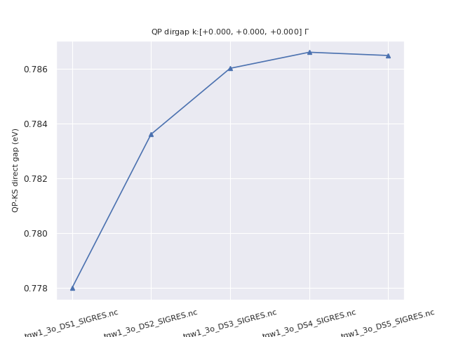
Invoking the script without options will open an ipython terminal to interact with the AbiPy robot. Use the -nb option to automatically generate a jupyter notebook that will open in your browser. For further details about the API provided by SigRes Robots see the Sigres notebook and the notebook with the GW lesson for GW calculations powered by AbiPy.

4 Convergence of the screening with respect to the number of bands

Now, we come back to the calculation of the screening. Adequate convergence studies will couple the change of parameters for optdriver = 3 with a computation of the GW energy changes. One cannot rely on the convergence of the macroscopic dielectric constant to assess the convergence of the GW energies.

As a consequence, we will define a double loop over the datasets:

ndtset      10
udtset      5  2

The datasets 12,22,32,42 and 52, drive the computation of the GW energies:

# Calculation of the Self-Energy matrix elements (GW corrections)
optdriver?2   4
getscr?2     -1
ecutsigx      8.0
nband?2       100

The datasets 11,21,31,41 and 51, drive the corresponding computation of the screening:

# Calculation of the screening (epsilon^-1 matrix)
optdriver?1  3

In this latter series, we will have to vary the two different parameters ecuteps and nband.

Let us begin with nband. This convergence study is rather important. It can be done at the same time as the convergence study for the number of bands for the self-energy. Note that the number of bands used to calculate both the screening and the self-energy can be lowered by a large amount by resorting to the extrapolar technique (see the input variable gwcomp).

Second, we check the convergence on the number of bands in the calculation of the screening. This will be done by defining five datasets, with increasing nband:

nband11  25
nband21  50
nband31  100
nband41  150
nband51  200

In directory Work_gw1, copy the file tgw1_4.abi:

    cp $ABI_TESTS/tutorial/Input/tgw1_4.abi .

Edit the tgw1_4.abi file, and take the time to examine it. Then, issue:

    cp tgw1_2o_DS2_WFK tgw1_4o_DS2_WFK
    abinit tgw1_4.abi > tgw1_4.log 2> err &

View tests/tutorial/Input/tgw1_4.abi

Edit the output file. The number of bands used for the wavefunctions in the computation of the screening is mentioned in the fragments of output:

     EPSILON^-1 parameters (SCR file):
     dimension of the eps^-1 matrix on file            169
     dimension of the eps^-1 matrix used               169
     number of plane-waves for wavefunctions           283
     number of bands                                    25

Gathering the GW energies for each number of bands, one gets:

  number of bands                                    25
        4   4.665 -11.412 -13.527   1.968   0.786  -0.273 -11.527  -0.115   4.550
        5   7.108  -9.962  -4.945  -4.279   0.796  -0.257  -9.375   0.587   7.696
  number of bands                                    50
        4   4.665 -11.412 -13.527   1.798   0.784  -0.275 -11.661  -0.248   4.417
        5   7.108  -9.962  -4.945  -4.446   0.789  -0.268  -9.512   0.451   7.559
  number of bands                                   100
        4   4.665 -11.412 -13.527   1.708   0.784  -0.276 -11.731  -0.318   4.347
        5   7.108  -9.962  -4.945  -4.523   0.791  -0.264  -9.571   0.391   7.499
  number of bands                                   150
        4   4.665 -11.412 -13.527   1.685   0.783  -0.276 -11.749  -0.336   4.329
        5   7.108  -9.962  -4.945  -4.542   0.790  -0.265  -9.586   0.376   7.485
  number of bands                                   200
        4   4.665 -11.412 -13.527   1.678   0.783  -0.277 -11.754  -0.341   4.324
        5   7.108  -9.962  -4.945  -4.549   0.790  -0.265  -9.592   0.370   7.479

So that the computation using 100 bands can be considered converged within 30 meV. Note that the value of nband that gives a converged dielectric matrix is usually of the same order of magnitude than the one that gives a converged \(\Sigma_c\).

5 Convergence of the screening matrix with respect to the number of planewaves

Then, we check the convergence on the number of plane waves in the calculation of the screening. This will be done by defining six datasets, with increasing ecuteps:

ecuteps:?     3.0
ecuteps+?     1.0

In directory Work_gw1, get the file tgw1_5.abi:

    cp $ABI_TESTS/tutorial/Input/tgw1_5.abi .

Edit the tgw1_5.abi file, and take the time to examine it. Then, issue:

    cp tgw1_2o_DS2_WFK tgw1_5o_DS2_WFK
    abinit tgw1_5.abi > tgw1_5.log 2> err &

View tests/tutorial/Input/tgw1_5.abi

Edit the output file. The number of bands used for the wavefunctions in the computation of the screening is mentioned in the fragments of output:

     EPSILON^-1 parameters (SCR file):
     dimension of the eps^-1 matrix                     59

Gathering the GW energies for each number of bands, one gets:

     dimension of the eps^-1 matrix                     59
        4   4.665 -11.412 -13.527   1.899   0.786  -0.272 -11.582  -0.169   4.496
        5   7.108  -9.962  -4.945  -4.462   0.791  -0.264  -9.523   0.440   7.548
     dimension of the eps^-1 matrix                    113
        4   4.665 -11.412 -13.527   1.755   0.784  -0.275 -11.694  -0.282   4.383
        5   7.108  -9.962  -4.945  -4.513   0.791  -0.264  -9.563   0.400   7.508
     dimension of the eps^-1 matrix                    137
        4   4.665 -11.412 -13.527   1.728   0.784  -0.276 -11.715  -0.303   4.362
        5   7.108  -9.962  -4.945  -4.518   0.791  -0.264  -9.567   0.395   7.504
     dimension of the eps^-1 matrix                    169
        4   4.665 -11.412 -13.527   1.708   0.784  -0.276 -11.731  -0.318   4.347
        5   7.108  -9.962  -4.945  -4.523   0.791  -0.264  -9.571   0.391   7.499
     dimension of the eps^-1 matrix                    259
        4   4.665 -11.412 -13.527   1.696   0.784  -0.276 -11.740  -0.328   4.338
        5   7.108  -9.962  -4.945  -4.527   0.791  -0.264  -9.574   0.388   7.496
     dimension of the eps^-1 matrix                    283
        4   4.665 -11.412 -13.527   1.695   0.784  -0.276 -11.741  -0.329   4.337
        5   7.108  -9.962  -4.945  -4.527   0.791  -0.264  -9.575   0.388   7.496

So that ecuteps = 6.0 (%npweps = 169) can be considered converged within 10 meV.

At this stage, we know that for the screening computation, we need ecuteps = 6.0 Ha and nband = 100.

Of course, until now, we have skipped the most difficult part of the convergence tests: the convergence in the number of k-points. It is as important to check the convergence on this parameter, than on the other ones. However, this might be very time consuming, since the CPU time scales as the square of the number of k-points (roughly), and the number of k-points can increase very rapidly from one possible grid to the next denser one. This is why we will leave this out of the present tutorial, and consider that we already know a sufficient k-point grid, for the last calculation.

As discussed in [Setten2017], the convergence study for k-points the number of bands and the cutoff energies can be decoupled in the sense that one can start from a reasonaby coarse k-mesh to find the converged values of nband, ecuteps, ecutsigx and then fix these values and look at the convergence with respect to the BZ mesh.

6 Calculation of the GW corrections for the band gap at the zone center

Now we try to perform a GW calculation for a real problem: the calculation of the GW corrections for the direct band gap of bulk silicon at the \(\Gamma\) point.

In directory Work_gw1, get the file tgw1_6.abi:

    cp $ABI_TESTS/tutorial/Input/tgw1_6.abi .

Then, edit the tgw1_6.abi file, and, without examining it, comment the line

     ngkpt    2 2 2    # Density of k points used for the automatic tests of the tutorial

and uncomment the line

    #ngkpt    4 4 4    # Density of k points needed for a converged calculation

Then, issue:

    abinit tgw1_6.abi > tgw1_6.log 2> err &

This job lasts a couple of minutes or so. It is worth to run it before the examination of the input file. Now, you can examine it.

View tests/tutorial/Input/tgw1_6.abi

We need the usual part of the input file to perform a ground state calculation. This is done in datasets 1 and 2. At the end of dataset 2, we print out the density and wavefunction files. We use a set of 19 k-points in the Irreducible Brillouin Zone. This set of k-points is not shifted so it contains the \(\Gamma\) point.

In dataset 3 we calculate the screening. The screening calculation is very time-consuming. So, we have decided to decrease a bit the parameters found in the previous convergence studies. Indeed, nband has been decreased from 100 to 50. The CPU time of this part is linear with respect to this parameter (or more exactly, with the number of conduction bands). Thus, the CPU time has been decreased by a factor of 2. Referring to our previous convergence study, we see that the absolute accuracy on the GW energies is now on the order of 0.2 eV only. This would be annoying for the absolute positioning of the band energy as required for band-offset or ionization potential of finite systems. However, as long as we are only interested in the gap energy that is fine enough.

Finally, in dataset 4, we calculate the self-energy matrix element at \(\Gamma\), using the previously determined parameters.

You should obtain the following results:

--- !SelfEnergy_ee
iteration_state: {dtset: 4, }
kpoint     : [   0.000,    0.000,    0.000, ]
spin       : 1
KS_gap     :    2.564
QP_gap     :    3.196
Delta_QP_KS:    0.632
data: !SigmaeeData |
     Band     E0 <VxcDFT>   SigX SigC(E0)      Z dSigC/dE  Sig(E)    E-E0       E
        2   4.369 -11.316 -12.769   0.817   0.765  -0.308 -11.803  -0.487   3.882
        3   4.369 -11.316 -12.769   0.817   0.765  -0.308 -11.803  -0.487   3.882
        4   4.369 -11.316 -12.769   0.817   0.765  -0.308 -11.803  -0.487   3.882
        5   6.933 -10.039  -5.840  -4.010   0.765  -0.307  -9.894   0.144   7.078
        6   6.933 -10.039  -5.840  -4.010   0.765  -0.307  -9.894   0.144   7.078
        7   6.933 -10.039  -5.840  -4.010   0.765  -0.307  -9.894   0.144   7.078
...

So that the DFT energy gap in \(\Gamma\) is about 2.564 eV, while the GW correction is about 0.632 eV, so that the GW band gap found is 3.196 eV.

One can compare now what have been obtained to what one can get from the literature.

     EXP         3.40 eV   Landolt-Boernstein

     DFT (LDA)
     LDA         2.57 eV   L. Hedin, Phys. Rev. 139, A796 (1965)
     LDA         2.57 eV   M.S. Hybertsen and S. Louie, PRL 55, 1418 (1985)
     LDA (FLAPW) 2.55 eV   N. Hamada, M. Hwang and A.J. Freeman, PRB 41, 3620 (1990)
     LDA (PAW)   2.53 eV   B. Arnaud and M. Alouani, PRB 62, 4464 (2000)
     LDA         2.53 eV   present work

     GW          3.27 eV   M.S. Hybertsen and S. Louie, PRL 55, 1418 (1985)
     GW          3.35 eV   M.S. Hybertsen and S. Louie, PRB 34, 5390 (1986)
     GW          3.30 eV   R.W. Godby, M. Schlueter, L.J. Sham, PRB 37, 10159 (1988)
     GW  (FLAPW) 3.30 eV   N. Hamada, M. Hwang and A.J. Freeman, PRB 41, 3620 (1990)
     GW  (FLAPW) 3.12 eV   W. Ku and A.G. Eguiluz, PRL 89, 126401 (2002)
     GW          3.20 eV   present work

The values are spread over an interval of 0.2 eV. They depend on the details of the calculations. In the case of pseudopotential calculations, they depend of course on the pseudopotential used. However, a GW result is hardly more accurate than 0.1 eV, in the present state of the art. But this goes also with the other source of inaccuracy, the choice of the pseudopotential, that can arrive up to even 0.2 eV. This can also be taken into account when choosing the level of accuracy for the convergence parameters in the GW calculation. As a reasonable target, the numerical sources of errors, due to insufficient ecuteps, nband, k point grid, should be kept lower than 0.02 or 0.03 eV.

7 How to compute GW band structures

Finally, it is possible to calculate a full GW band plot of a system via interpolation. There are three possible techniques.

The first one is based on the use of Wannier functions to interpolate a few selected points in the IBZ obtained using the direct GW approach [Hamann2009]. You need to have the Wannier90 plug-in installed. See the directory tests/wannier90, test case 03, for an example of a file where a GW calculation is followed by the use of Wannier90.

View tests/wannier90/Input/t03.abi

The wannier interpolation is a very accurate method, can handle band crossings but it may require additional work to obtain well localized wannier functions. Another practical way follows from the fact that the QP energies, similarly to the KS eigenvalues, must fulfill the symmetry properties:

\[ \ee(\kpG) = \ee(\kk) \]

and

\[ \ee(S\kk) = \ee(\kk) \]

where \(\GG\) is a reciprocal lattice vector and \(S\) is a rotation of the point group of the crystal. Therefore it’s possible to employ the star-function interpolation by Shankland, Koelling and Wood [Euwema1969], [Koelling1986] in the improved version proposed by [Pickett1988] to fit the ab-initio results. This interpolation technique, by construction, passes through the initial points and satisfies the basic symmetry property of the band energies. It should be stressed, however, that this Fourier-based method can have problems in the presence of band crossings that may cause unphysical oscillations between the ab-initio points. To reduce this spurious effect, we suggest to interpolate the GW corrections instead of the GW energies. The corrections, indeed, are usually smoother in k-space and the resulting fit is more stable. A python example showing how to construct an interpolated scissor operator with AbiPy is available here

The third method uses the fact that the GW corrections are usually linear with the energy, for each group of bands. This is evident when reporting on a plot the GW correction with respect to the 0-order KS energy for each state. One can then simply correct the KS band structure at any point, by using a GW correction for the k-points where it has not been calculated explicitly, using a fit of the GW correction at a sparse set of points. A python example showing how to construct an energy-dependent scissor operator with AbiPy is available here.

8 Advanced features of GW calculations

The user might switch to the second GW tutorial before coming back to the present section.

Calculations without using the Plasmon-Pole model

In order to circumvent the plasmon-pole model, the GW frequency convolution has to be calculated explicitly along the real axis. This is a tough job, since G and W have poles along the real axis. Therefore it is more convenient to use another path of integration along the imaginary axis plus the residues enclosed in the path.

Consequently, it is better to evaluate the screening for imaginary frequencies (to perform the integration) and also for real frequencies (to evaluate the contributions of the residues that may enter into the path of integration). The number of imaginary frequencies is set by the input variable nfreqim. The regular grid of real frequencies is determined by the input variables nfreqre, which sets the number of real frequencies, and freqremax, which indicates the maximum real frequency used.

The method is particularly suited to output the spectral function (contained in file out.sig). The grid of real frequencies used to calculate the spectral function is set by the number of frequencies (input variable nfreqsp) and by the maximum frequency calculated (input variable freqspmax).

Self-consistent calculations

The details in the implementation and the justification for the approximations retained can be found in [Bruneval2006]. The only added input variables are getqps and irdqps. These variables concerns the reading of the _QPS file, that contains the eigenvalues and the unitary transform matrices of a previous quasiparticle calculation. QPS stands for “QuasiParticle Structure”.

The only modified input variables for self-consistent calculations are gwcalctyp and bdgw. When the variable gwcalctyp is in between 0 and 9, The code calculates the quasiparticle energies only and does not output any QPS file (as in a standard GW run). When the variable gwcalctyp is in between 10 and 19, the code calculates the quasiparticle energies only and outputs them in a QPS file. When the variable gwcalctyp is in between 20 and 29, the code calculates the quasiparticle energies and wavefunctions and outputs them in a QPS file.

For a full self-consistency calculation, the quasiparticle wavefunctions are expanded in the basis set of the KS wavefunctions. The variable bdgw now indicates the size of all matrices to be calculated and diagonalized. The quasiparticle wavefunctions are consequently linear combinations of the KS wavefunctions in between the min and max values of bdgw.

A correct self-consistent calculation should consist of the following runs:

• 1) Self-consistent KS calculation: outputs a WFK file
• 2) Screening calculation (with KS inputs): outputs a SCR file
• 3) Sigma calculation (with KS inputs): outputs a QPS file
• 4) Screening calculation (with the WFK, and QPS file as an input): outputs a new SCR file
• 5) Sigma calculation (with the WFK, QPS and the new SCR files): outputs a new QPS file
• 6) Screening calculation (with the WFK, the new QPS file): outputs a newer SCR file
• 7) Sigma calculation (with the WFK, the newer QPS and SCR files): outputs a newer QPS
• ............ and so on, until the desired accuracy is reached

Note that for Hartree-Fock calculations a dummy screening is required for initialization reasons. Therefore, a correct HF calculations should look like

• 1) Self-consistent KS calculation: outputs a WFK file
• 2) Screening calculation using very low convergence parameters (with KS inputs): output a dummy SCR file
• 3) Sigma calculation (with KS inputs): outputs a QPS file
• 4) Sigma calculation (with the WFK and QPS files): outputs a new QPS file
• 5) Sigma calculation (with the WFK and the new QPS file): outputs a newer QPS file
• ............ and so on, until the desired accuracy is reached

In the case of a self-consistent calculation, the output is slightly more complex: For instance, at iteration 2

--- !SelfEnergy_ee
iteration_state: {dtset: 3, }
kpoint     : [   0.500,    0.250,    0.000, ]
spin       : 1
KS_gap     :    3.684
QP_gap     :    5.764
Delta_QP_KS:    2.080
data: !SigmaeeData |
     Band     E_DFT   <VxcDFT>   E(N-1)  <Hhartree>   SigX  SigC[E(N-1)]    Z     dSigC/dE  Sig[E(N)]  DeltaE  E(N)_pert E(N)_diago
        1    -3.422   -10.273    -3.761     6.847   -15.232     4.034     1.000     0.000   -11.198    -0.590    -4.351    -4.351
        2    -0.574   -10.245    -0.850     9.666   -13.806     2.998     1.000     0.000   -10.807    -0.291    -1.141    -1.141
        3     2.242    -9.606     2.513    11.841   -11.452     1.931     1.000     0.000    -9.521    -0.193     2.320     2.320
        4     3.595   -10.267     4.151    13.866   -11.775     1.842     1.000     0.000    -9.933    -0.217     3.934     3.934
        5     7.279    -8.804     9.916    16.078    -4.452    -1.592     1.000     0.000    -6.044     0.119    10.034    10.035
        6    10.247    -9.143    13.462    19.395    -4.063    -1.775     1.000     0.000    -5.838     0.095    13.557    13.557
        7    11.488    -9.704    15.159    21.197    -4.061    -1.863     1.000     0.000    -5.924     0.113    15.273    15.273
        8    11.780    -9.180    15.225    20.958    -3.705    -1.893     1.000     0.000    -5.598     0.135    15.360    15.360
...

The columns are

• Band: Index of the band
• E_DFT: DFT eigenvalue
• VxcDFT: Diagonal expectation value of the xc potential in between DFT bra and ket
• E(N-1): Quasiparticle energy of the previous iteration (equal to DFT for the first iteration)
• Hhartree: Diagonal expectation value of the Hartree Hamiltonian (equal to E_DFT - VxcDFT for the first iteration only)
• SigX: Diagonal expectation value of the exchange self-energy
• SigC[E(N-1)]: Diagonal expectation value of the correlation self-energy (evaluated for the energy of the preceeding iteration)
• Z: Quasiparticle renormalization factor Z (taken equal to 1 in methods HF, SEX, COHSEX and model GW)
• dSigC/dE: Derivative of the correlation self-energy with respect to the energy
• Sig[E(N)]: Total self-energy for the new quasiparticle energy
• DeltaE: Energy difference with respect to the previous step
• E(N)_pert: QP energy as obtained by the usual perturbative method
• E(N)_diago: QP energy as obtained by the full diagonalization