Parallelism for the ground state using wavelets
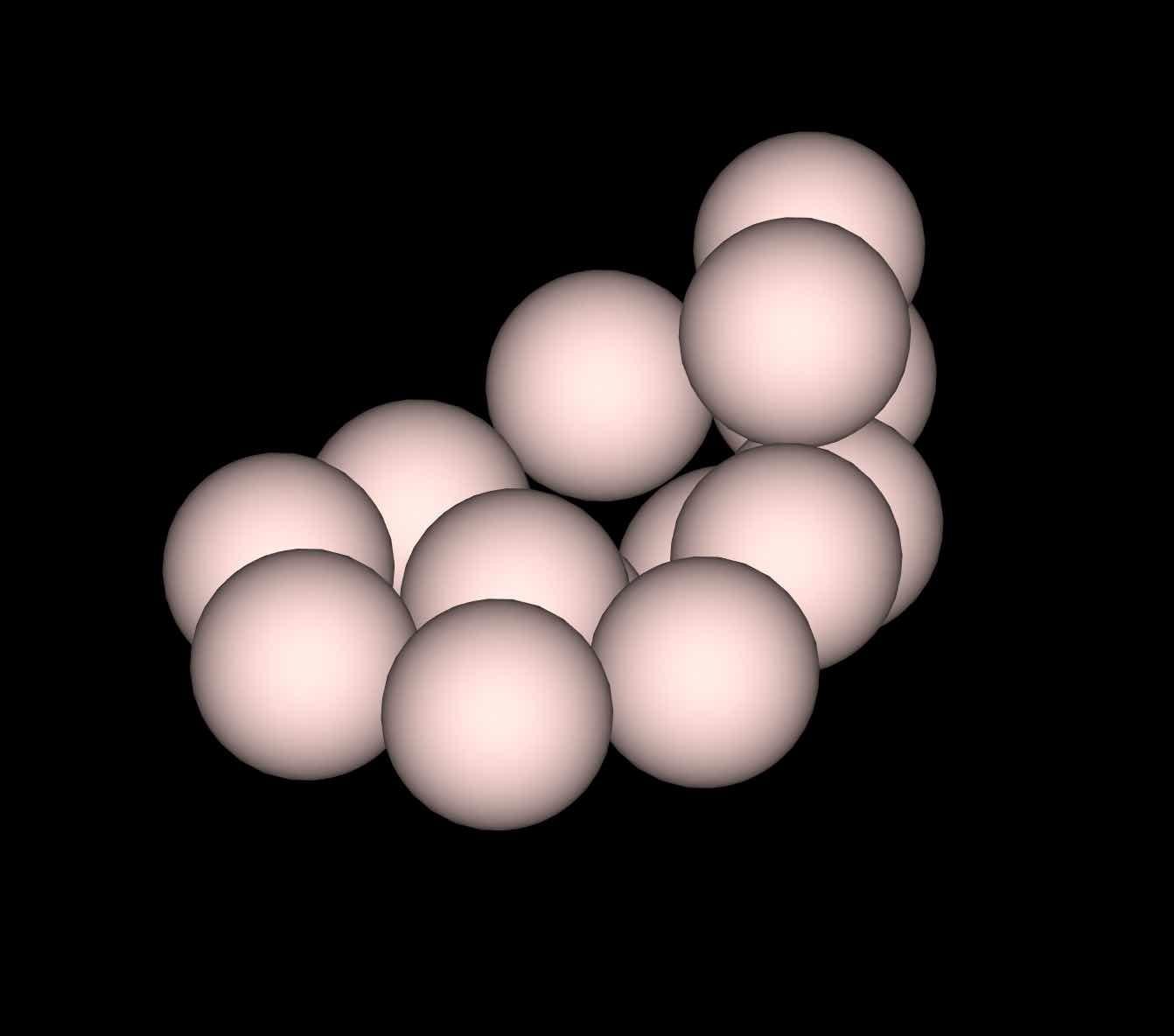
Boron cluster, alkane molecule…
This tutorial explains how to run the calculation of an isolated system using a wavelet basis-set on a parallel computer using MPI. You will learn the different characteristics of a parallel run using the wavelet basis-set and test the speed-up on a small boron cluster of 14 atoms followed by a test on a bigger alkane molecule.
This tutorial should take about 90 minutes and requires you have several CPU cores (up to 64 if possible).
You are supposed to know already some basics of parallelism in ABINIT, explained in the tutorial A first introduction to ABINIT in parallel.
The tutorial will be more profitable if you have already performed calculations using the wavelet formalism (see the topic page on wavelets and the usewvl keyword).
Important
To use a wavelet basis set ABINIT should have been compiled with the bigdft library.
To do this, download the bigdft fallback and use
the --with-bigdft, BIGDFT_LIBS, BIGDFT_FCFLAGS, etc. flags during the
configure step.
Note
Supposing you made your own installation of ABINIT, the input files to run the examples are in the ~abinit/tests/ directory where ~abinit is the absolute path of the abinit top-level directory. If you have NOT made your own install, ask your system administrator where to find the package, especially the executable and test files.
In case you work on your own PC or workstation, to make things easier, we suggest you define some handy environment variables by executing the following lines in the terminal:
export ABI_HOME=Replace_with_absolute_path_to_abinit_top_level_dir # Change this line
export PATH=$ABI_HOME/src/98_main/:$PATH      # Do not change this line: path to executable
export ABI_TESTS=$ABI_HOME/tests/             # Do not change this line: path to tests dir
export ABI_PSPDIR=$ABI_TESTS/Pspdir/  # Do not change this line: path to pseudos dir
Examples in this tutorial use these shell variables: copy and paste
the code snippets into the terminal (remember to set ABI_HOME first!) or, alternatively,
source the set_abienv.sh script located in the ~abinit directory:
source ~abinit/set_abienv.sh
The ‘export PATH’ line adds the directory containing the executables to your PATH so that you can invoke the code by simply typing abinit in the terminal instead of providing the absolute path.
To execute the tutorials, create a working directory (Work*) and
copy there the input files of the lesson.
Most of the tutorials do not rely on parallelism (except specific tutorials on parallelism). However you can run most of the tutorial examples in parallel with MPI, see the topic on parallelism.
1 Wavelets variables and parallelism
The parallelism with the wavelet formalism can be used for two purposes: to reduce the memory load per node, or to reduce the overall computation time.
The MPI parallelization in the wavelet mode relies on the orbital distribution
scheme, in which the orbitals of the system under investigation are
distributed over the assigned MPI processes. This scheme reaches its limit
when the number of MPI processes is equal to the number of orbitals in the
simulation. To distribute the orbitals uniformly, the number of processors
must be a factor (divisor) of the number of orbitals. If this is not the case,
the distribution is not optimal, but the code tries to balance the load over
the processors. For example, if we have 5 orbitals and 4 processors, the
orbitals will have the distribution: 2/1/1/1.
There are no specific input variables to use the parallelism in the wavelet
mode as the only parallelisation level is on orbitals. So running ABINIT with
an mpirun command is enough (this command differs according to the local MPI
implementation) such as:
mpirun -n Nproc abinit < infile.abi >& logfile
For further understanding of the wavelet mode, or for citation purposes, one may read [Genovese2008]
2 Speed-up calculation for a boron cluster
We propose here to determine the speed-up in the calculation of the total energy of a cluster made of 14 boron atoms.
Open the file tgswvl_1.abi. It
contains first the definition of the wavelet basis-set. One may want to test
the precision of the calculation by varying the wvl_hgrid and
wvl_crmult variables. This is not the purpose of this tutorial, so we will
use the given values (0.45 Bohr and 5).
# Input for PARAL_GSWVL tutorial
# 14 atom boron cluster, parallel calculation

#-------------------------------------------------------------------------------
#Definition of variables specific to a wavelet calculation

usewvl       1    # Activation of the "wavelet" basis set

wvl_hgrid 0.45    # Wavelet H step grid
wvl_crmult   5    # Wavelet coarse grid radius multiplier
wvl_frmult   8    # Wavelet fine grid radius multiplier

icoulomb     1    # Activate the free boundary conditions for the
                  # Hartree potential computation, done in real space.
                  # This is the value to choose for molecules in the wavelet formalism.

iscf         0    # Activation of the Direct minimization scheme for the calculation
                  #   of wavefunctions. This algorithm is fast but working only for
                  #   systems with a gap, and only for wavelets.

nwfshist     6    # Activation of DIIS algoithm (Direct minimization scheme)
                  #   with 6 wavefunctions stored in history

timopt      10    # This will create a YAML file with the timings of the WVL routines

#-------------------------------------------------------------------------------

#Definition of the unit cell
acell 3*20        # Lengths of the primitive vectors (big box to isolate the molecule)
                  # Primitive vectors are not given here  (rprim)
                  #   because "cubic" is the default value

#Definition of the atom types and pseudopotentials
ntypat 1          # There is only one type of atom
znucl 5           # Atomic number of the possible type(s) of atom. Here boron.
pp_dirpath "$ABI_PSPDIR"        # Path to the directory were
                                #   pseudopotentials for tests are stored
pseudos "B-q3"                  # Name and location of the pseudopotential

#Definition of the atoms
natom 14          # There are 14 atoms
typat 14*1        # They all are of type 1, that is, Carbon
xcart             # Location of the atoms, given in cartesian coordinates (angstrom):
 6.23174441376337462  11.10650949517181125   8.80369514094791228
 6.46975493123427281  11.64662037074667290   7.38942614477337933
 6.06260066201525571   9.92651732450364754   7.48967117179688202
 7.80101706261892769  10.57816432104265840   7.83061522324544157
 6.31690262930086011   8.31702761150885550   7.01500573994981380
 7.75164346206343247   7.71450195176475972   8.07490331742471490
 7.03603095641418808   9.37653827161064335   6.05099299166473248
 9.17770300902474467   7.98319528851733384   8.99010444257574015
 7.16405045957283093  10.88564910545551710   6.23700501567613319
 7.62758557507984225   5.97498074889332820   7.97176704264589375
 7.14341418637742454  10.01632171818918770   9.42744042423526629
 8.44317230240882566   9.32780744990434307   8.78315808382683194
 6.51462241221419625   6.81056643770915038   7.30106028716855171
 8.83833328151791164   6.50337987446461785   8.70844982986595006

#k point grid definition
#  We set the grid manually to impose a computation at Gamma point
#  (only available value for a molecule)
kptopt  0         # Option for manual setting of k-points
istwfk *1         # No time-reversal symmetry optimization (not compatible with WVL)
nkpt    1         # Number of k-points (here only gamma)
kpt  3*0.         # - K-point coordinates in reciprocal space

#Parameters for the SCF procedure
nstep 20          # Maximal number of SCF cycles
tolwfr 1.0d-14    # Will stop when, twice in a row, the difference
                  # between two consecutive evaluations of wavefunction residual
                  # differ by less than tolwfr
                  # This convergence criterion is adapted to direct minimization
                  #   algorithm (iscf=0)

#Miscelaneous parameters
prtwf 0           # Do not print wavefunctions
prtden 0          # Do not print density
prteig 0          # Do not print eigenvalues
optstress 0       # Stress tensor computation is not relevant here


##############################################################
# This section is used only for regression testing of ABINIT #
##############################################################
#%%<BEGIN TEST_INFO>
#%% [setup]
#%% executable = abinit
#%% need_cpp_vars = HAVE_BIGDFT
#%% [files]
#%% [paral_info]
#%% max_nprocs = 14
#%% nprocs_to_test = 1, 2, 4, 8, 10, 12
#%% [NCPU_1]
#%% files_to_test = tgswvl_1_MPI1.abo, tolnlines =   3, tolabs =  1.1e-5, tolrel= 1.1e-4
#%% [NCPU_2]
#%% files_to_test = tgswvl_1_MPI2.abo, tolnlines =   3, tolabs =  1.1e-5, tolrel= 1.1e-4
#%% [NCPU_4]
#%% files_to_test = tgswvl_1_MPI4.abo, tolnlines =   3, tolabs =  1.1e-5, tolrel= 1.1e-4
#%% [NCPU_8]
#%% files_to_test = tgswvl_1_MPI8.abo, tolnlines =   3, tolabs =  1.1e-5, tolrel= 1.1e-4
#%% [NCPU_10]
#%% files_to_test = tgswvl_1_MPI10.abo, tolnlines =   4, tolabs =  1.1e-4, tolrel= 1.1e-4
#%% [NCPU_12]
#%% files_to_test = tgswvl_1_MPI12.abo, tolnlines =   3, tolabs =  1.1e-5, tolrel= 1.1e-4
#%% [extra_info]
#%% authors = D. Caliste
#%% keywords = NC,WVL
#%% description =
#%%   Input for PARAL_GSWVL tutorial
#%%   14 atom boron cluster, parallel calculation
#%%<END TEST_INFO>
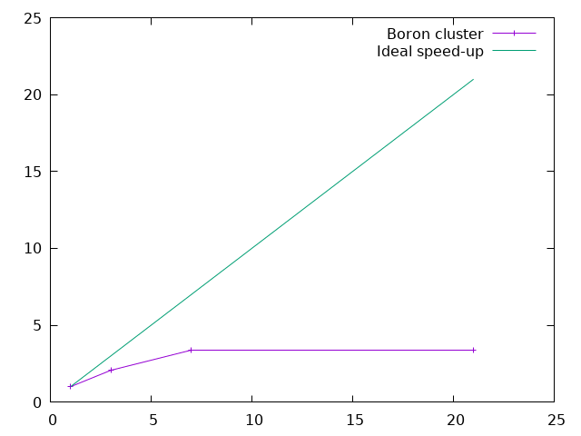
Run ABINIT with 3 processors. The overall time is printed at the end of the output file (and of the log):
Proc. 0 individual time (sec): cpu= 36.0 wall= 36.0
Read the output file to find the number of orbitals in the calculation (given by the keyword nband). With the distribution scheme of the wavelet mode, the best distribution over processors will be obtained for, 1, 3, 7 and 21 processors. Create four different directories (with the number of processors for instance) and run four times ABINIT with the same input file, varying the number of processors in {1, 3, 7, 21}.
abinit tgswvl_1.abi >& log
The speed-up is the ratio between the time with one processor and the time of a run with N processors.
Assuming that the directories are called {01, 03, 07, 21}, one can grep the
over-all time of a run and plot it with the gnuplot graphical tool.
Just issue:
gnuplot
and, in gnuplot command line, type:
plot "< grep 'individual time' */*.abo | tr '/' ' '" u 1:(ttt/$11) w lp t "Boron cluster", x t "Ideal speed-up"
where ttt represents the time on one processor (replace ttt by this time in the
command line above).
The efficiency (in percent) of the parallelization process is the ratio between the speed-up and the number of processors. One can plot it (using gnuplot) with:
plot "< grep 'individual time' */*.abo | tr '/' ' '" u 1:(ttt/$11/$1*100) w lp t "Boron cluster"
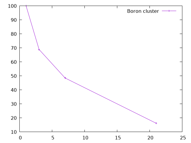
The first conclusion is that the efficiency is not so good when one use one orbital per processor. This is a general rule with the wavelet mode: due to the implementation, a good balance between speed and efficiency is obtained for two orbitals per processor. One can also see that the efficiency generally decreases with the number of processors.
This system is rather small and the amount of time spent in the overhead (read the input file, initialise arrays…) is impacting the performance. Let’s see how to focus on the calculation parts.
3 Time partition
The wavelet mode is generating a wvl_timings.yml file at each run (warning: it will
erase any existing copy). This is a text file in YAML format
that can be read directly. There are three sections, giving the time of the initialisation
process (sectionINITS), the time of the SCF loop itself (section WFN OPT),
and the time for the post-processing (section POSTPRC).
Note
The wvl_timings.yaml file is only created if timopt
is set to 10 in the input file.
Let’s have a closer look to the SCF section. We can extract the following data (the actual figures will vary between runs and number of processors):
== WFN OPT:
 #  Class                    % , Time (s),   Max, Min Load (relative)
 Flib LowLevel         : [  6.8,      1.7,  1.16,  0.84]
 Communications        : [ 33.3,      8.1,  1.16,  0.85]
 BLAS-LAPACK           : [  0.1, 3.63E-02,  1.09,  0.91]
 PS Computation        : [  5.4,      1.3,  1.03,  0.89]
 Potential             : [  7.3,      1.8,  1.17,  0.58]
 Convolutions          : [ 42.4,      10.,  1.10,  0.88]
 Linear Algebra        : [  0.1, 3.61E-02,  1.03,  0.98]
 Other                 : [  1.3,     0.33,  1.23,  0.77]
 Initialization        : [  0.1, 2.64E-02,  1.35,  0.81]
 Total                 : [ 96.9,      24.,  1.00,  1.00]

 # Category                  % ,  Time (s),   Max, Min Load (relative)
  Allreduce, Large Size: [ 22.7,       5.5,  1.23,  0.88]
    Class              : Communications, Allreduce operations
  Rho_comput           : [ 16.9,       4.1,  1.19,  0.79]
    Class              : Convolutions, OpenCL ported
  Precondition         : [ 13.0,       3.2,  1.01,  0.99]
    Class              : Convolutions, OpenCL ported
  ApplyLocPotKin       : [ 12.6,       3.1,  1.08,  0.89]
    Class              : Convolutions, OpenCL ported
  Exchange-Correlation : [  7.3,       1.8,  1.17,  0.58]
    Class              : Potential, construct local XC potential
  PSolver Computation  : [  5.4,       1.3,  1.03,  0.89]
    Class              : PS Computation, 3D SG_FFT and related operations
  Init to Zero         : [  4.1,       1.0,  1.17,  0.78]
    Class              : Flib LowLevel, Memset of storage space
  Allreduce, Small Size: [  3.4,      0.84,  1.89,  0.26]
    Class              : Communications, Allreduce operations
  Pot_commun           : [  3.2,      0.79,  1.08,  0.93]
    Class              : Communications, AllGathrv grid
  PSolver Communication: [  2.4,      0.59,  1.21,  0.96]
    Class              : Communications, MPI_ALLTOALL and MPI_ALLGATHERV
  Array allocations    : [  2.3,      0.55,  1.16,  0.89]
    Class              : Flib LowLevel, Heap storage allocation
  Un-TransComm         : [  1.1,      0.27,  1.07,  0.92]
    Class              : Communications, ALLtoALLV
  Diis                 : [  0.7,      0.16,  1.24,  0.75]
    Class              : Other, Other
  ApplyProj            : [  0.5,      0.11,  1.10,  0.89]
    Class              : Other, RMA pattern
  Rho_commun           : [  0.4,  9.42E-02,  6.63,  0.02]
    Class              : Communications, AllReduce grid
  Vector copy          : [  0.4,  8.59E-02,  1.56,  0.69]
    Class              : Flib LowLevel, Memory copy of arrays
  Un-TransSwitch       : [  0.2,  5.99E-02,  1.65,  0.59]
    Class              : Other, RMA pattern
  Blas GEMM            : [  0.1,  3.62E-02,  1.09,  0.91]
    Class              : BLAS-LAPACK, Matrix-Matrix multiplications
  Chol_comput          : [  0.1,  3.58E-02,  1.03,  0.98]
    Class              : Linear Algebra, ALLReduce orbs
  CrtLocPot            : [  0.1,  2.64E-02,  1.35,  0.81]
    Class              : Initialization, Miscellaneous
  Routine Profiling    : [  0.1,  1.32E-02,  1.07,  0.90]
    Class              : Flib LowLevel, Profiling performances
With the total time of this WFN OPT section, one can compute the speed-up and the
efficiency of the wavelet mode more accurately:
  N processors   Time (s)   Speed-up  Efficiency (%)
       3           40.        2.1        69.2
       7           24.        3.5        49.4
      21           20.        4.2        19.8
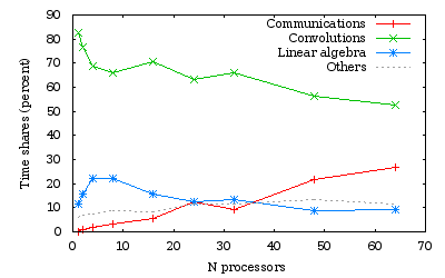
With the percentages of the wvl_timings.yaml file, one can see that, for this
example, the time is mostly spent in communications, the precondionner,
the computation of the density and the application of the local part of the Hamiltonian.
Let’s categorise the time information:
- The communication time (all entries of class
Communications). - The time spent doing convolutions (all entries of class
Convolutions). - The linear algebra part (all entries of class
Linear AlgebraandBLAS-LAPACK). - The other entries are in miscellaneous categories.
The summations are given in the file, on top of the section. One obtains the percentage per category during the SCF loop:
 CLASS            PERCENT    TIME(sec)
 Convolutions      42.4        10.0
 Communications    33.3         8.1
 Potential          7.3         1.8
 Flib Lowlevel      6.8         1.7
 PS Computation     5.4         1.3
 Linear Algebra     0.2         0.1
 Other              4.6         1.8
You can analyse all the wvl_timings.yaml that have been generated for the different
number of processors and see the evolution of the different categories.
4 Orbital parallelism and array parallelism
If the number of processors is not a divisor of the number of orbitals, there will be some processors with fewer orbitals than others. This is not the best distribution from an orbital point of view. But, the wavelet mode also distributes the scalar arrays like density and potentials by z-planes in real space. So some parts of the code may become more efficient when used with a bigger number of processors, like the Poisson Solver part for instance.
Run the boron example with {2, 4, 14, 15} processors and plot the speed-up.
One can also look at the standard output to the load balancing of orbitals and the load balancing of the Poisson Solver (with 15 processors):
With 15 processors the repartition of the 21 orbitals is the following:
 Processes from 0  to  9 treat 2 orbitals
 Processes from 10 to 10 treat 1 orbitals
 Processes from 11 to 14 treat 0 orbitals
With 15 processors, we can read in log file:
[...]
 Poisson Kernel Initialization:
   MPI tasks                           :  15
 Poisson Kernel Creation:
   Boundary Conditions                 : Free
   Memory Requirements per MPI task:
     Density (MB)                      :  1.33
     Kernel (MB)                       :  1.40
     Full Grid Arrays (MB)             :  18.18
     Load Balancing of calculations:
       Density:
         MPI tasks 0- 14               : 100%
       Kernel:
         MPI tasks 0- 13               : 100%
         MPI task 14                   :  50%
       Complete LB per task            : 1/3 LB_density + 2/3 LB_kernel
[...]
As expected, one can see that:
-
The load balancing per orbital is bad (4 processors are doing nothing)
-
The load balancing of the scalar arrays distribution is not so good since the last processor will have a reduced array.
It is thus useless to run this job at 15 processors; 14 will give the same run time (since the load balancing will be better).
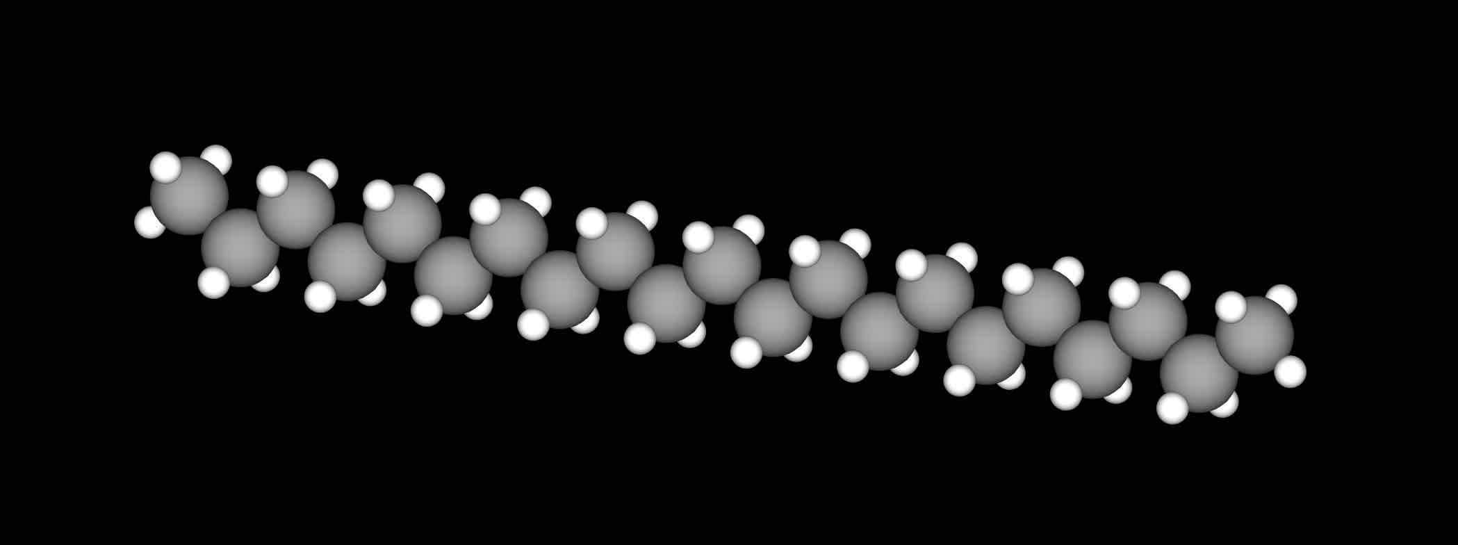
5 Speed-up calculation on a 65-atom alkane
Let’s do the same with a bigger molecule and a finer grid. Open the file
tgswvl_2.abi. It contains the definition of an alkane chain of 65 atoms,
providing 64 orbitals.
# Input for PARAL_GSWVL tutorial
# 65-atom alkane chain of 65 atoms, parallel calculation

#-------------------------------------------------------------------------------
#Definition of variables specific to a wavelet calculation

usewvl       1    # Activation of the "wavelet" basis set

wvl_hgrid 0.30    # Wavelet H step grid
wvl_crmult   7    # Wavelet coarse grid radius multiplier
wvl_frmult   8    # Wavelet fine grid radius multiplier

icoulomb     1    # Activate the free boundary conditions for the
                  # Hartree potential computation, done in real space.
                  # This is the value to choose for molecules in the wavelet formalism.

iscf         2    # Activation of the simple mixing scheme for the density.

nwfshist     6    # Activation of DIIS algoithm for the calculation of wavefunctions
                  #   (Direct minimization scheme)
                  #   with 6 wavefunctions stored in history

timopt      10    # This will create a YAML file with the timings of the WVL routines

#-------------------------------------------------------------------------------

#Definition of the unit cell
acell 3*100       # Lengths of the primitive vectors (big box to isolate the molecule)
                  # Primitive vectors are not given here  (rprim)
                  #   because "cubic" is the default value
nsym 1            # Do not use symmetries (not relevant here)

#Definition of the atom types and pseudopotentials
ntypat 2          # There is only one type of atom
znucl 6 1         # Atomic number of the possible type(s) of atom. Here boron, hydrogen.
pp_dirpath "$ABI_PSPDIR"    # Path to the directory were
                            #   pseudopotentials for tests are stored
pseudos "C-q4, H-q1"        # Name and location of the pseudopotentials

#Definition of the atoms
natom 65          # There are 65 atoms
typat 21*1 44*2   # 21 are of type 1 (carbon), 44 are of type 2 (hydrogen)
xcart             # Location of the atoms, given in cartesian coordinates (angstrom):
  0.00000    0.00000    0.00000
  0.00000    0.88250    1.24804
  0.00000    0.00000    2.49609
  0.00000    0.88250    3.74413
  0.00000    0.00000    4.99217
  0.00000    0.88250    6.24022
  0.00000    0.00000    7.48826
  0.00000    0.88250    8.73630
  0.00000    0.00000    9.98435
  0.00000    0.88250   11.23239
  0.00000    0.00000   12.48043
  0.00000    0.88250   13.72848
  0.00000    0.00000   14.97652
  0.00000    0.88250   16.22457
  0.00000    0.00000   17.47261
  0.00000    0.88250   18.72065
  0.00000    0.00000   19.96870
  0.00000    0.88250   21.21674
  0.00000    0.00000   22.46478
  0.00000    0.88250   23.71283
  0.00000    0.00000   24.96087
  0.00000    0.61775   -0.87363
  0.87363   -0.61775    0.00000
 -0.87363   -0.61775    0.00000
  0.87363    1.50025    1.24804
 -0.87363    1.50025    1.24804
  0.87363   -0.61775    2.49609
 -0.87363   -0.61775    2.49609
  0.87363    1.50025    3.74413
 -0.87363    1.50025    3.74413
  0.87363   -0.61775    4.99217
 -0.87363   -0.61775    4.99217
  0.87363    1.50025    6.24022
 -0.87363    1.50025    6.24022
  0.87363   -0.61775    7.48826
 -0.87363   -0.61775    7.48826
  0.87363    1.50025    8.73630
 -0.87363    1.50025    8.73630
  0.87363   -0.61775    9.98435
 -0.87363   -0.61775    9.98435
  0.87363    1.50025   11.23239
 -0.87363    1.50025   11.23239
  0.87363   -0.61775   12.48043
 -0.87363   -0.61775   12.48043
  0.87363    1.50025   13.72848
 -0.87363    1.50025   13.72848
  0.87363   -0.61775   14.97652
 -0.87363   -0.61775   14.97652
  0.87363    1.50025   16.22457
 -0.87363    1.50025   16.22457
  0.87363   -0.61775   17.47261
 -0.87363   -0.61775   17.47261
  0.87363    1.50025   18.72065
 -0.87363    1.50025   18.72065
  0.87363   -0.61775   19.96870
 -0.87363   -0.61775   19.96870
  0.87363    1.50025   21.21674
 -0.87363    1.50025   21.21674
  0.87363   -0.61775   22.46478
 -0.87363   -0.61775   22.46478
  0.87363    1.50025   23.71283
 -0.87363    1.50025   23.71283
  0.87363   -0.61775   24.96087
 -0.87363   -0.61775   24.96087
  0.00000    0.61775   25.83450
  Angstrom

#k point grid definition
#  We set the grid manually to impose a computation at Gamma point
#  (only available value for a molecule)
kptopt  0         # Option for manual setting of k-points
istwfk *1         # No time-reversal symmetry optimization (not compatible with WVL)
nkpt    1         # Number of k-points (here only gamma)
kpt  3*0.         # - K-point coordinates in reciprocal space

#Parameters for the SCF procedure
nstep 20          # Maximal number of SCF cycles
tolwfr 1.0d-4     # Will stop when, twice in a row, the difference
                  # between two consecutive evaluations of wavefunction residual
                  # differ by less than tolwfr
                  # This convergence criterion is adapted to direct minimization
                  #   algorithm (iscf=0)

#Miscelaneous parameters
prtwf 0           # Do not print wavefunctions
prtden 0          # Do not print density
prteig 0          # Do not print eigenvalues
optstress 0       # Stress tensor computation is not relevant here


##############################################################
# This section is used only for regression testing of ABINIT #
##############################################################
#%%<BEGIN TEST_INFO>
#%% [setup]
#%% executable = abinit
#%% need_cpp_vars = HAVE_BIGDFT
#%% [files]
#%% files_to_test =
#%% [paral_info]
#%% max_nprocs = 64
#%% nprocs_to_test = 24, 32, 48
#%% [NCPU_24]
#%% files_to_test = tgswvl_2_MPI24.abo, tolnlines =   0, tolabs =  0.0, tolrel= 0.0
#%% [NCPU_32]
#%% files_to_test = tgswvl_2_MPI32.abo, tolnlines =   0, tolabs =  0.0, tolrel= 0.0
#%% [NCPU_48]
#%% files_to_test = tgswvl_2_MPI48.abo, tolnlines =   0, tolabs =  0.0, tolrel= 0.0
#%% [extra_info]
#%% authors = D. Caliste
#%% keywords = NC,WVL
#%% description =
#%%   Input for PARAL_GSWVL tutorial
#%%   65-atom alkane chain of 65 atoms, parallel calculation
#%%   WARNING : This test might not be functional anymore.
#%%   It has not been tested since the final v10.3.0 of ABINIT due to unexplained failure
#%%   at the merge between v10.2.2 and previous commits in v10.3.0, both working.
#%%<END TEST_INFO>
Run this input file with {1, 2, 4, 8, 16, 24, 32, 48, 64} processors. The run with one processor should take less than one hour. If the time is short, one can reduce wvl_hgrid in the input file to 0.45.
Time measurements for a run over several processors of a \(C_{21}H_{44}\) alkane chain
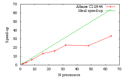
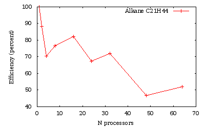
As we obtained previously, the efficiency is generally lowered when the number of processors is not a divisor of the number of orbitals (namely here 24 and 48).
6 Conclusion
With the wavelet mode, it is possible to efficiently decrease the run time by increasing the number of processors. The efficiency is limited by the increase of amount of time spent in the communications. The efficiency increases with the quality of the calculation: the more accurate the calculations are (finer hgrid…), the more efficient the code parallelization will be.