Third tutorial on the Projector Augmented-Wave (PAW) technique
Testing PAW datasets against an all-electron code
This tutorial will demonstrate how to test a generated PAW dataset against an
all-electron code. We will be comparing results with the open Elk FP-LAPW code
(a branch of the EXCITING code) available under GPLv3.
You will learn how to compare calculations of the equilibrium lattice
parameter, the Bulk modulus and the band structure between ABINIT PAW results
and those from the Elk code.
It is assumed you already know how to use ABINIT in the PAW case. The tutorial
assumes no previous experience with the Elk code, but it is strongly advised
that the users familiarise themselves a bit with this code before attempting
to do similar comparisons with their own datasets.
This tutorial should take about 3h-4h.
Note
Supposing you made your own installation of ABINIT, the input files to run the examples are in the ~abinit/tests/ directory where ~abinit is the absolute path of the abinit top-level directory. If you have NOT made your own install, ask your system administrator where to find the package, especially the executable and test files.
In case you work on your own PC or workstation, to make things easier, we suggest you define some handy environment variables by executing the following lines in the terminal:
export ABI_HOME=Replace_with_absolute_path_to_abinit_top_level_dir # Change this line
export PATH=$ABI_HOME/src/98_main/:$PATH      # Do not change this line: path to executable
export ABI_TESTS=$ABI_HOME/tests/             # Do not change this line: path to tests dir
export ABI_PSPDIR=$ABI_TESTS/Pspdir/  # Do not change this line: path to pseudos dir
Examples in this tutorial use these shell variables: copy and paste
the code snippets into the terminal (remember to set ABI_HOME first!) or, alternatively,
source the set_abienv.sh script located in the ~abinit directory:
source ~abinit/set_abienv.sh
The ‘export PATH’ line adds the directory containing the executables to your PATH so that you can invoke the code by simply typing abinit in the terminal instead of providing the absolute path.
To execute the tutorials, create a working directory (Work*) and
copy there the input files of the lesson.
Most of the tutorials do not rely on parallelism (except specific tutorials on parallelism). However you can run most of the tutorial examples in parallel with MPI, see the topic on parallelism.
1. Introduction - the quantities to be compared
When comparing results between all-electron and pseudopotential codes, it is usually impossible to compare total energies. This is because the total energy of an all-electron code includes the contribution from the kinetic energy of the core orbitals, while in the pseudopotential approach, the only information that is retained is the density distribution of the frozen core. This is typically so even in a PAW implementation.
Differences in total energies should be comparable, but calculating these to a given accuracy is usually a long and cumbersome process. However, some things can be calculated with relative ease. These include structural properties - such as the equilibrium lattice parameter(s) and the bulk modulus - as well as orbital energies, i.e. the band structure for a simple bulk system.
Note
We are here aiming to compare the results under similar numerical conditions. That does not necessarily mean that the calculations can be compared with experimental results, nor that the results of the calculations individually represent the absolutely most converged values for a given system. However, to ensure that the numerical precision is equivalent, we must take care to:
- Use the same (scalar-relativistic) exchange-correlation functional.
- Match the
Elkmuffin-tin radii and the PAW cutoff radii. - Use a k-point grid of similar quality.
- Use a similar cutoff for the plane wave expansion.
- Freeze the core in the
Elkcode (whenever possible), to match the frozen PAW core inABINIT. - Use a similar atomic on-site radial grid.
We will use Carbon, in the diamond structure, as an example of a simple solid with a band gap, and we will use Magnesium as an example of a metallic solid. Naturally, it is important to keep things as simple as possible when benchmarking PAW datasets, and there is a problem when the element has no naturally occurring pure solid phase. For elements which are molecular in their pure state (like Oxygen, Nitrogen and so forth), or occur only in compound solids, one solution is to compare results on a larger range of solids where the other constituents have already been well tested. For instance, for oxygen, one could compare results for ZnO, MgO and MnO, provided that one has already satisfied oneself that the datasets for Zn, Mg, and Mn in their pure forms are good.
One could also compare results for molecules, and we encourage you to do this
if you have the time. However, doing this consistently in ABINIT requires a
supercell approach and would make this tutorial very long, so we shall not do
it here. We will now discuss the prerequisites for this tutorial.
2. Prerequisites, code components and scripts
It is assumed that you are already familiar with the contents and procedures
in tutorials PAW1 and PAW2, and so
have some familiarity with input files for ATOMPAW , and the issues in creating
PAW datasets. To exactly reproduce the results in this tutorial, you will
need:
- The
ATOMPAWcode for generating PAW datasets (see tutorial PAW2, section 2.).
       cd atompaw-4.x.y.z
       mkdir build
       cd build
       ../configure
       make
-
the
Elkcode (this tutorial was designed with v1.2.15), available here. We will use theElkcode itself, as well as itseos(equation-of-state) utility, for calculating equilibrium lattice parameters. -
Auxiliary
bashandpythonscripts for the comparison of band structures, available in the directory $ABI_HOME/doc/tutorial/paw3_assets/scripts/. For thepythonscripts,python3is required. There are also various gnuplot scripts there.
You will of course also need a working copy of ABINIT. Please make sure that
the above components are downloaded and working on your system before
continuing this tutorial. The tutorial also makes extensive use of gnuplot , so
please also ensure that a recent and working version is installed on your system.
Note
By the time that you are doing this tutorial there will probably be newer versions of all these programs available. It is of course better to use the latest versions, and we simply state the versions of codes used when this tutorial was written so that specific numerical results can be reproduced if necessary.
3. Carbon (diamond)
3.1. Carbon - a simple datatset
Make a working directory for the ATOMPAW generation (you could call it
C_atompaw) and copy the file: C_simple.input to it.
C 6                                         ! Atomic name and number
LDA-PW scalarrelativistic loggrid 801 logderivrange -10 40 1000 ! XC approx., SE type, gridtype, # pts, logderiv
2 2 0 0 0 0                                 ! maximum n for each l: 2s,2p,0d,0f..
2 1 2                                       ! Partially filled shell: 2p^2
0 0 0                                       ! Stop marker
c                                           ! 1s - core
v                                           ! 2s - valence
v                                           ! 2p - valence
1                                           ! l_max treated = 1
1.3                                         ! core radius r_c
n                                           ! no more unoccupied s-states
n                                           ! no more unoccupied p-states
vanderbilt                                  ! vanderbilt scheme for finding projectors
2 0                                         ! localisation scheme
1.3                                         ! Core radius for occ. 2s state
1.3                                         ! Core radius for occ. 2p state
XMLOUT                                      ! Run atompaw2abinit converter
prtcorewf noxcnhat nospline noptim          ! XML conversion options
END                                         ! Exit
Then go there and run ATOMPAW by typing (assuming that you have set things up so that you
can run atompaw by just typing atompaw):
atompaw < C_simple.input
The code should run, and if you do an ls, the contents of the directory will be something like:
 C                        density     logderiv.2  potSC1   tprod.2  wfn2    wfnSC1
 C.LDA-PW-paw.xml         dummy       NC          rvf      vloc     wfn3
 C.LDA-PW-paw.xml.corewf  fort.24     OCCWFN      rVx      wfn001   wfn4
 compare.abinit           logderiv.0  potAE0      tau      wfn002   wfn5
 C_simple.input           logderiv.1  potential   tprod.1  wfn1     wfnAE0
There is a lot of output, so it is useful to work with a graphical overview.
Copy the gnuplot script plot_C_all.p to your folder.
Open a new terminal window by typing xterm &, and run gnuplot in the new
terminal window. At the gnuplot command prompt type:
gnuplot> load 'plot_C_all.p'
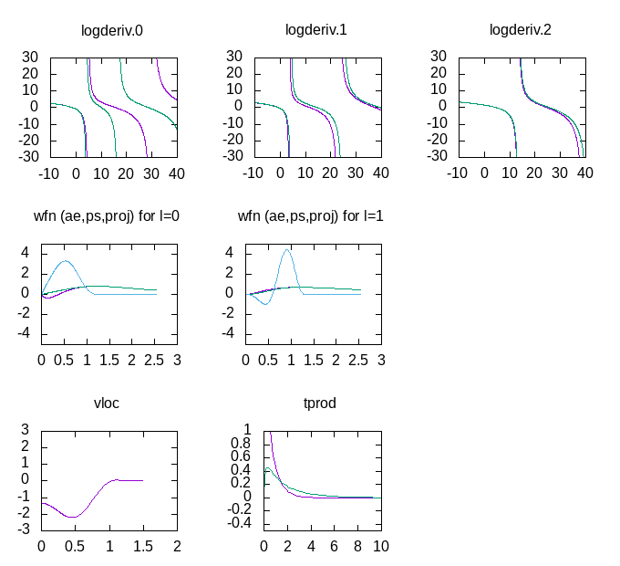
You should get a plot that looks like this:
You can now keep the gnuplot terminal and plot window open as you work, and if
you change the ATOMPAW input file and re-run it, you can update the plot by
retyping the load.. command. The gnuplot window plots the essential
information from the ATOMPAW outputs, the logarithmic derivatives, (the
derivatives of the dataset are green), the wavefunctions and projectors for
each momentum channel (the full wavefunction is in red, the PW part is green,
and the projector is blue) as well as the local potential. Finally, it shows the Fourier transform
of the projector products (the x-axis is in units of Ha).
The inputs directory also contains scripts for plotting these graphs
individually, and you are encouraged to test and modify them. We can look
inside the C_simple.input file:
C 6                                         ! Atomic name and number
LDA-PW scalarrelativistic loggrid 801 logderivrange -10 40 1000 ! XC approx., SE type, gridtype, # pts, logderiv
2 2 0 0 0 0                                 ! maximum n for each l: 2s,2p,0d,0f..
2 1 2                                       ! Partially filled shell: 2p^2
0 0 0                                       ! Stop marker
c                                           ! 1s - core
v                                           ! 2s - valence
v                                           ! 2p - valence
1                                           ! l_max treated = 1
1.3                                         ! core radius r_c
n                                           ! no more unoccupied s-states
n                                           ! no more unoccupied p-states
vanderbilt                                  ! vanderbilt scheme for finding projectors
2 0                                         ! localisation scheme
1.3                                         ! Core radius for occ. 2s state
1.3                                         ! Core radius for occ. 2p state
XMLOUT                                      ! Run atompaw2abinit converter
prtcorewf noxcnhat nospline noptim          ! XML conversion options
END                                         ! Exit
Here we see that the current dataset is very simple, it has no basis states
beyond the \(2s\) and \(2p\) occupied valence states in carbon. It is thus not
expected to produce very good results, since there is almost no flexibility in
the PAW dataset. Note that the scalarrelativistic option is turned on. While
this is not strictly necessary for such a light atom, we must always ensure to
have this turned on if we intend to compare with results from the Elk code.
We will now run basic convergence tests in ABINIT for this dataset. The
dataset file for ABINIT has already been generated (it is the C.LDA-PW-paw.xml
file in the current directory). Make a new subdirectory for the
test in the current directory (you could call it abinit_test for instance), go
there and copy the file: ab_C_test.abi into
it. This ABINIT input file contains several datasets which increment the ecut
input variable, and perform ground state and band structure calculations for
each value of ecut. This is thus the internal ABINIT convergence study. Any
dataset is expected to converge to a result sooner or later, but that does not
mean that the final result is accurate, unless the dataset is good. The goal
is of course to generate a dataset which both converges quickly and is very accurate.
# Input for PAW3 tutorial
# C - diamond structure

#-------------------------------------------------------------------------------
#Directories and files

pseudos="C.LDA-PW-paw.xml"

pp_dirpath="../"
outdata_prefix="outputs/ab_C_test_o"
tmpdata_prefix="outputs/ab_C_test"


#-------------------------------------------------------------------------------
#Define the different datasets

ndtset 18       # 18 double-index datasets
udtset 9 2      # 1st index running from 1 to 9 and the 2nd from 1 to 2

#Cutoff variables
ecut:?  5.0
ecut+?  5.0
pawecutdg 110.0
ecutsm 0.5

#Dataset 1
#Ground-state run
chksymbreak 0
kptopt?1  1
nshiftk?1 1
shiftk?1  0.5 0.5 0.5
ngkpt     10 10 10
tolvrs?1 1.0d-14
nstep?1  150
getwfk21 11
getwfk31 21
getwfk41 31
getwfk51 41
getwfk61 51
getwfk71 61
getwfk81 71
getwfk91 81
nbdbuf?1 4
nband?1  8

#Dataset 2
#Definition of the k-point grid
#the band structure
iscf?2    -2
getden?2  -1
kptopt?2  -4
nband?2    8
nbdbuf?2   0
ndivk?2    8 10 6 10 # divisions of the 6 segments
kptbounds?2
           0.5  0.5  0.5  #L
           0.0  0.0  0.0  #Gamma
           0.5  0.0  0.5  #X
           0.75 0.5  0.75 #U
           0.0  0.0  0.0  #Gamma

tolwfr?2  1.0d-18
enunit?2  0             # Will output the eigenenergies in Ha
nstep?2 150


#-------------------------------------------------------------------------------
#Definition of the Unit cell

#Definition of the unit cell
acell 3*6.7403
rprim
   0.5  0.5  0.0
   0.0  0.5  0.5
   0.5  0.0  0.5

#Definition of the atom types
ntypat 1          # One tom type
znucl 6           # Carbon

#Definition of the atoms
natom 2           # 2 atoms per cell
typat 1 1         # each of type carbon
xred              # This keyword indicates that the location of the atoms
                  # will follow, one triplet of number for each atom
   0.125    0.125    0.125
  -0.125   -0.125   -0.125


#-------------------------------------------------------------------------------
#Miscelaneous

#GS convergence fix
istwfk *1
The ab_C_test.abi file contains:
pseudos="C.LDA-PW-paw.xml"

pp_dirpath="../"
outdata_prefix="outputs/ab_C_test_o"
tmpdata_prefix="outputs/ab_C_test"
So it expects the newly generated dataset to be in the directory above.
Also, to keep things tidy, it assumes the outputs will be put in a subdirectory
called outputs/. Make sure to create it before you start the ABINIT run by writing:
mkdir outputs
Important
You may have to change the path to reach the Pspdir repository. For this, modify the variable pp_dirpath in the input file.
You can now run the ABINIT tests (maybe even in a separate new xterm window), by executing:
abinit ab_C_test.abi >& log_C_test
There are 18 double-index datasets in total, with the first index running from
1 to 9 and the second from 1 to 2. You can check on the progress of the
calculation by issuing ls outputs/. When the .._o_DS92.. files appear, the
calculation should be just about finished. While the calculation runs you
might want to take a look in the input file. Note the lines pertaining to the
increment in ecut (around line 29):
 ...
 #Cutoff variables
 ecut:? 5.0
 ecut+?  5.0
 `pawecutdg` 110.0
 ecutsm 0.5
 ...
ecut is increased in increments of 5 Ha from an initial value of 5, to a final
ecut of 45 Ha. Note that pawecutdg is kept fixed, at a value high enough to be
expected to be good for the final value of ecut. In principle, a convergence
study of pawecutdg should be performed as well, once a good value of ecut has been found.
We can now check the basic convergence attributes of the dataset. The
convergence of the total energy is easily checked by issuing some grep commands:
grep 'etotal' ab_C_test.abo
This should give you an output similar to this (though not the text to the left):
                                     etotal   (ecut)
 etotal11 -1.0972441353E+01
 etotal21 -1.1443217299E+01      - 470.78 mHa (10 Ha)
 etotal31 -1.1507234681E+01      -  64.02 mHa (15 Ha)
 etotal41 -1.1517560274E+01      -  10.33 mHa (20 Ha)
 etotal51 -1.1518066800E+01      -   0.51 mHa (25 Ha)
 etotal61 -1.1518201844E+01      -   0.14 mHa (30 Ha)
 etotal71 -1.1518427967E+01      -   0.23 mHa (35 Ha)
 etotal81 -1.1518542165E+01      -   0.11 mHa (40 Ha)
 etotal91 -1.1518570692E+01      -   0.03 mHa (45 Ha)
Your values might differ slightly in the last decimals. The calculation of
diamond with the current PAW Carbon dataset converged to a precision of the
total energy below 1 mHa for a cutoff of about 25 Ha (this is not particularly
good for a PAW dataset). Also, the convergence is a bit jumpy after an ecut of
about 25 Ha, which is an indication of a) that the number of projectors per
angular momentum channel is low, and b) that other parameters apart from ecut
dominate convergence beyond this point.
If we turn to the band structure, we can use the script
comp_bands_abinit2abinit.py
to check the convergence of the band structure. Copy the script to the
directory where the ABINIT input file is and issue:
python comp_bands_abinit2abinit.py outputs/ab_C_test_o_DS12_EIG outputs/ab_C_test_o_DS92_EIG eV
This will print a long series of columns and at the end you will see:
 ...
 #        nvals:   280
 # average diff:     1.758809  eV
 # minimum diff:    -4.437905  eV
 # maximum diff:     1.089000  eV
 #
 # NOTE: `ABINIT` values are read in fixed format with five decimal
 #       places. For low values, four or three decimal figures
 #       may be the highest precision you can get.
This provides you with some statistics of the difference in the band energies.
Specifically this is the average difference between a the band structure
calculated at an ecut of 5 Ha (in dataset 12) and another at an ecut of 45 Ha (in dataset 92).
The differences between these datasets are naturally very large, about 1.8 eV on average, because the band-structure of the first dataset is far from converged. The columns output before the statistics are arranged so that if you pipe the output to a data file:
python comp_bands_abinit2abinit.py outputs/ab_C_test_o_DS12_EIG outputs/ab_C_test_o_DS92_EIG eV > bands_5Ha_vs_45Ha.dat
you can plot the two band structures in gnuplot directly, by entering:
gnuplot> plot 'bands_5Ha_vs_45Ha.dat' u 1:2 w lp title '5 Ha', 'bands_5Ha_vs_45Ha.dat' u 1:3 w lp title '45 Ha'
This should furnish you with a graph that looks something like this:
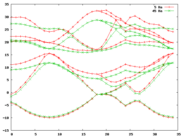
Not surprisingly, the band structures are very different. However, a search
through the datasets of increasing index (i.e. DS22, DS32, DS42, …) yields
that for dataset 42, i.e with an ecut of 20 Ha, we are already converged to a
level of 0.01 eV. Issuing the command:
python comp_bands_abinit2abinit.py outputs/ab_C_test_o_DS42_EIG outputs/ab_C_test_o_DS92_EIG eV > bands_20Ha_vs_45Ha.dat
and plotting this with:
gnuplot> plot 'bands_20Ha_vs_45Ha.dat' u 1:2 w lp title '20 Ha', 'bands_20Ha_vs_45Ha.dat' u 1:3 w lp title '45 Ha'
Should give you a plot similar to this:
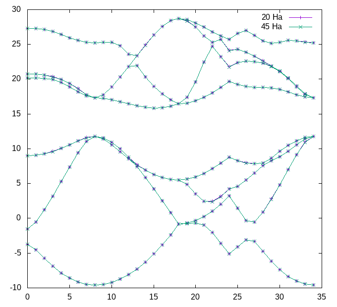
You can convince yourself by zooming in that the band structures are very similar. The statistics at the end of the bands_20Ha_vs_45Ha.dat file shows that we are converged within abinit:
...
#        nvals:   280
# average diff:     0.003808  eV
# minimum diff:    -0.008980  eV
# maximum diff:     0.000272  eV
...
3.2. Carbon - calculating the equilibrium lattice parameter
That we have converged the dataset on its own does of course not mean that the
dataset is good, i.e. that it reproduces the same results as an all-electron
calculation. To independently verify that the dataset is good, we need to
calculate the equilibrium lattice parameter (and the Bulk modulus) and compare
this and the band structure with an Elk calculation.
First, we will need to calculate the total energy of diamond in ABINIT for a
number of lattice parameters around the minimum of the total energy. There is
example input file for doing this at:
ab_C_equi.abi.
The new input file has ten datasets which increment the lattice parameter, alatt,
from 6.1 to 7.0 Bohr in steps of 0.1 Bohr. A look in the input file will tell
you that ecut is set to 25 Hartrees. Copy these to your abinit_test directory and run:
# Input for PAW3 tutorial
# C - diamond structure

#-------------------------------------------------------------------------------
#Directories and files

pseudos="C.LDA-PW-paw.xml"

pp_dirpath="../"
outdata_prefix="outputs/ab_C_equi_o"
tmpdata_prefix="outputs/ab_C_equi"


#-------------------------------------------------------------------------------
#Define the different datasets

ndtset 10            # 10 datasets
acell: 3*6.1  Bohr   # The starting values of the cell parameters
acell+ 3*0.1  Bohr   # The increment of acell from one dataset to the other


#-------------------------------------------------------------------------------
#Convergence parameters

#Cutoff variables
ecut 25.0
pawecutdg 110.0
ecutsm 0.5

#Definition of the k-point grid
chksymbreak 0
kptopt 1
nshiftk 1
shiftk 0.5 0.5 0.5
ngkpt 10 10 10

#Bands and occupations
nband  8
nbdbuf 4

#SCF cycle parameters
tolvrs 1.0d-10
nstep  150


#-------------------------------------------------------------------------------
#Definition of the Unit cell

#Definition of the unit cell
acell 3*6.7403
rprim
   0.5  0.5  0.0
   0.0  0.5  0.5
   0.5  0.0  0.5

#Definition of the atom types
ntypat 1          # One tom type
znucl 6           # Carbon

#Definition of the atoms
natom 2           # 2 atoms per cell
typat 1 1         # each of type carbon
xred              # This keyword indicates that the location of the atoms
                  # will follow, one triplet of number for each atom
   0.125    0.125    0.125
  -0.125   -0.125   -0.125
abinit ab_C_equi.abi >& log_C_equi
The run should be done fairly quickly, and when it’s done we can check on the volume and the total energy by using “grep”
grep 'volume' log_C_equi
and
grep 'etotal' log_C_equi
The outputs should be something like this:
 ...
 Unit cell volume ucvol=  5.6745250E+01 bohr^3
 Unit cell volume ucvol=  5.9582000E+01 bohr^3
 Unit cell volume ucvol=  6.2511750E+01 bohr^3
 Unit cell volume ucvol=  6.5536000E+01 bohr^3
 Unit cell volume ucvol=  6.8656250E+01 bohr^3
 Unit cell volume ucvol=  7.1874000E+01 bohr^3
 Unit cell volume ucvol=  7.5190750E+01 bohr^3
 Unit cell volume ucvol=  7.8608000E+01 bohr^3
 Unit cell volume ucvol=  8.2127250E+01 bohr^3
 Unit cell volume ucvol=  8.5750000E+01 bohr^3
 ...
       etotal1    -1.1461991605E+01
       etotal2    -1.1480508012E+01
       etotal3    -1.1494820912E+01
       etotal4    -1.1505365819E+01
       etotal5    -1.1512537944E+01
       etotal6    -1.1516696065E+01   <-
       etotal7    -1.1518166172E+01   <- minimum around here
       etotal8    -1.1517244861E+01   <-
       etotal9    -1.1514202226E+01
       etotal10   -1.1509284702E+01
 ...
If we examine the etotal values, the total energy does indeed go to a
minimum, and we also see that given the magnitude of the variations of the
total energy, an ecut of 25 Ha should be more than sufficient. We will now
extract the equilibrium volume and bulk modulus by using the eos bundled with
elk. This requires us to put the above data in an eos.in file. Create such a
file with your favorite editor and enter the following five lines and then the
data you just extracted:
 "C - Diamond"                : cname - name of material
 2                            : natoms - number of atoms
 1                            : etype - equation of state fit type
 50.0 95.0 100                : vplt1, vplt2, nvplt - start, end and #pts for fit
 10                            : nevpt - number of supplied points
 5.6745250E+01  -1.1461991605E+01
 5.9582000E+01  -1.1480508012E+01
 6.2511750E+01  -1.1494820912E+01
 6.5536000E+01  -1.1505365819E+01
 6.8656250E+01  -1.1512537944E+01
 7.1874000E+01  -1.1516696065E+01
 7.5190750E+01  -1.1518166172E+01
 7.8608000E+01  -1.1517244861E+01
 8.2127250E+01  -1.1514202226E+01
 8.5750000E+01  -1.1509284702E+01
When you run eos (the executable should be located in src/eos/ in the
directory where Elk was compiled), it will produce several .OUT files. The
file PARAM.OUT contains the information we need:
 C - Diamond

 Universal EOS
 Vinet P et al., J. Phys.: Condens. Matter 1, p1941 (1989)

 (Default units are atomic: Hartree, Bohr etc.)

 V0                =            75.50730327
 E0                =           -11.51817590
 B0                =           0.1564766690E-01
 B0'               =            3.685291965

 B0 (GPa)          =            460.3701770
This tells us the equilibrium volume and bulk modulus. The volume of our diamond FCC lattice depends on the lattice parameter as: \(\frac{a^3}{4}\). If we want to convert the volume to a lattice parameter, we have to multiply by four and then take the third root, so:
alatt = (4*75.50730327)^(1/3) = 6.7094 Bohr (3.5505 Å)
at equilibrium for this dataset.
3.3. Carbon - the all-electron calculation
In order to estimate whether these values are good or not, we need independent
verification, and this will be provided by the all-electron Elk code. There is
an Elk input file matching our ABINIT diamond calculation at
elk_C_diamond.in. You need
to copy this file to a directory set up for the Elk run (why not call it
C_elk), and it needs to be renamed to elk.in, which is the required input
name for an Elk calculation. We are now ready to run the Elk code for the first time.
If we take a look in the elk.in file, at the beginning we will see the lines:
 ! Carbon, diamond structure (FCC)

 ! The tasks keyword defines what will be done by the code:
 ! 0 - Perform ground-state calculation from scratch
 ! 1 - Restart GS calc. from STATE.OUT file
 ! 20 - Calculate band structure as defined by plot1d
 tasks
 0
 20

 ! Set core-valence cutoff energy
 ecvcut
  -6.0

 ! Construct atomic species file 'C.in'
 species
  6  : atomic number
  'C'
  'carbon'
  21894.16673    : atomic mass
  1.300000000    : muffin-tin radius
  4              : number of occ. states
  1   0   1   2  : 1s
  2   0   1   2  : 2s
  2   1   1   1  : 2p m=1
  2   1   2   1  : 2p m=2
...
! Carbon, diamond structure (FCC)

! The tasks define what will be done by the code:
! 0 - Perform ground-state calculation from scratch
! 1 - Restart GS calc. from STATE.OUT file
! 20 - Calculate band structure as defined by plot1d
tasks
0
20

! Set core-valence cutoff energy
ecvcut
 -6.0

! Construct atomic species file 'C.in'
! (comment this if you hve modified 'C.in')
species
   6  : atomic number
 'C'
 'carbon'
   21894.16673    : atomic mass
   1.300000000    : muffin-tin radius
   4              : number of occ. states
   1   0   1   2  : 1s
   2   0   1   2  : 2s
   2   1   1   1  : 2p m=1
   2   1   2   1  : 2p m=2

! Tolerance on convegence of band energies (absolute)
epsband
 1.e-8

! Tolerance on conv. of potential (relative)
epspot
 1.e-8

! Tolerance on conv. of total energy (absolute)
epsengy
 1.e-6

! Use adaptive linear mixing of densities
! 1 - Adaptive linear
! 2 - Pulay mixing
mixtype
 3

! Exchange-correlation functional to use
! LDA (PW92) is 3 (default) (equiv. Abinit ixc 7)
! GGA-PBE    is 20          (equiv. Abinit ixc 11)
! (see Elk manual for other options)
xctype
 3

! Define lattice vectors (FCC diamond has an
! experimental lattice parameter of 3.567 angstrom)
scale
 6.7403 : lattice parameter in Bohr

avec
     0.5  0.5  0.0
     0.0  0.5  0.5
     0.5  0.0  0.5

! Define atomic species
atoms
   1   : nspecies - Number of species
'C.in' : spfname - Name of species file
   2   : natoms; atposl, bfcmt below - Atoms in cell, reduced coord. and moments
    0.00000000    0.00000000    0.0000000    0.00000000  0.00000000  0.00000000
    0.25000000    0.25000000    0.2500000    0.00000000  0.00000000  0.00000000

! Set muffin-tin radius automatically
autormt
 .false.

! Freeze core states (in abinit PAW, they are frozen)
frozencr
 .true.

! Path to atomic data files
sppath
  './'

! Monkhorst-pack k-point grid
ngridk
 9  9  9

! Shift of MP grid
vkloff
0.5 0.5 0.5

! Set upper limit of |G+k|, the number below is
! (MT radius)*max(|G+k|)
rgkmax
8.0

! A value of 0.0 makes this being set automatically
gmaxvr
0.0

! k-points in band plot (this is copied from the k-point list
! reported by ABINIT in oreder to have a one-to-one correspondence)
plot1d
35 35  : nvp1d, npp1d
                     5.00000000E-01  5.00000000E-01  5.00000000E-01
                     4.37500000E-01  4.37500000E-01  4.37500000E-01
                     3.75000000E-01  3.75000000E-01  3.75000000E-01
                     3.12500000E-01  3.12500000E-01  3.12500000E-01
                     2.50000000E-01  2.50000000E-01  2.50000000E-01
                     1.87500000E-01  1.87500000E-01  1.87500000E-01
                     1.25000000E-01  1.25000000E-01  1.25000000E-01
                     6.25000000E-02  6.25000000E-02  6.25000000E-02
                     0.00000000E+00  0.00000000E+00  0.00000000E+00
                     5.00000000E-02  0.00000000E+00  5.00000000E-02
                     1.00000000E-01  0.00000000E+00  1.00000000E-01
                     1.50000000E-01  0.00000000E+00  1.50000000E-01
                     2.00000000E-01  0.00000000E+00  2.00000000E-01
                     2.50000000E-01  0.00000000E+00  2.50000000E-01
                     3.00000000E-01  0.00000000E+00  3.00000000E-01
                     3.50000000E-01  0.00000000E+00  3.50000000E-01
                     4.00000000E-01  0.00000000E+00  4.00000000E-01
                     4.50000000E-01  0.00000000E+00  4.50000000E-01
                     5.00000000E-01  0.00000000E+00  5.00000000E-01
                     5.41666667E-01  8.33333333E-02  5.41666667E-01
                     5.83333333E-01  1.66666667E-01  5.83333333E-01
                     6.25000000E-01  2.50000000E-01  6.25000000E-01
                     6.66666667E-01  3.33333333E-01  6.66666667E-01
                     7.08333333E-01  4.16666667E-01  7.08333333E-01
                     7.50000000E-01  5.00000000E-01  7.50000000E-01
                     6.75000000E-01  4.50000000E-01  6.75000000E-01
                     6.00000000E-01  4.00000000E-01  6.00000000E-01
                     5.25000000E-01  3.50000000E-01  5.25000000E-01
                     4.50000000E-01  3.00000000E-01  4.50000000E-01
                     3.75000000E-01  2.50000000E-01  3.75000000E-01
                     3.00000000E-01  2.00000000E-01  3.00000000E-01
                     2.25000000E-01  1.50000000E-01  2.25000000E-01
                     1.50000000E-01  1.00000000E-01  1.50000000E-01
                     7.50000000E-02  5.00000000E-02  7.50000000E-02
                     0.00000000E+00  0.00000000E+00  0.00000000E+00

! Number of empty bands to include
nempty
4

! Ratio betwen fine and coarse radial grid
! (the coarse grid is used for the calcualation
!  of densities). This needs to be set to one
! so that the grid specified in the .in file
! of the atomic species is used everywhere
lradstp
 1       : coarse/fine radial grid ratio
Any text after an exclamation mark (or a colon on the lines defining data) is
a comment. The keyword tasks defines what the code should do. In this case
it is set to calculate the ground state for the given structure and to
calculate a band structure. The block ecvcut sets the core-valence cutoff
energy. The next input block, species defines the parameters for the
generation of an atomic species file (it will be given the name C.in). As a
first step, we need to generate this file, but we will need to modify it
before we perform the main calculation. Therefore, you should run the code
briefly (by just running the executable in your directory) and then kill it
after a few seconds (using Ctrl+C for instance ), as soon as it has generated the C.in file.
If you look in your directory after the code has been killed you will probably
see a lot of .OUT files with uppercase names. These are the Elk output files.
You should also see a C.in file. When you open it, you should see:
 'C'                                        : spsymb
 'carbon'                                   : spname
  -6.00000                                  : spzn
   39910624.45                              : spmass
   0.816497E-06    1.3000   38.0877   300    : rminsp, rmt, rmaxsp, nrmt
   4                                        : nstsp
   1   0   1   2.00000    T                 : nsp, lsp, ksp, occsp, spcore
   2   0   1   2.00000    F
   2   1   1   1.00000    F
   2   1   2   1.00000    F
   1                                        : apword
    0.1500   0  F                           : apwe0, apwdm, apwve
   0                                        : nlx
   3                                        : nlorb
   0   2                                    : lorbl, lorbord
    0.1500   0  F                           : lorbe0, lorbdm, lorbve
    0.1500   1  F
   1   2                                    : lorbl, lorbord
    0.1500   0  F                           : lorbe0, lorbdm, lorbve
    0.1500   1  F
   0   2                                    : lorbl, lorbord
    0.1500   0  F                           : lorbe0, lorbdm, lorbve
   -0.5012   0  T
The first four lines contain information pertaining to the symbol, name, charge and mass of the atom. The fifth line holds data concerning the numerical grid: the distance of the first grid point from the origin, the muffin-tin radius, the maximum radius for the on-site atomic calculation, and the number of grid points. The subsequent lines contain data about the occupied states (the ones ending with “T” or “F”), and after that there is information pertaining to the FP-LAPW on-site basis functions.
The first important thing to check here is whether all the orbitals that we have included as valence states in the PAW dataset are treated as valence in this species file. We do this by checking that there is an “F” after the corresponding states in the occupation list:
 ...
    1   0   1   2.00000    T                 : spn, spl, spk, spocc, spcore
    2   0   1   2.00000    F
    2   1   1   1.00000    F
    2   1   2   1.00000    F
 ...
The first two numbers are the \(n\), \(l\) quantum numbers of the atomic state, so we see that the \(2s\) states, and the \(2p\) states are set to valence as in the PAW dataset.
Note
This might not be the case in general, the version of Elk we use is
modified to accept an adjustment of the cutoff energy for determining whether
a state should be treated as core or valence. This is what is set by the line:
...
ecvcut
-6.0 : core-valence cutoff energy
...
in the elk.in file. If you find too few or too many states are included as
valence for another atomic species, this value needs to be adjusted downwards or upwards.
The second thing we need to check is whether the number of grid points and the
muffin-tin radius that we use in the Elk calculation is roughly equivalent to
the PAW one. If you have a look in the PAW dataset we generated before, i.e.
in the C.LDA-PW-paw.xml file, there is the line:
   ...
   <radial_grid eq="r=a*(exp(d*i)-1)" a=" 2.1888410558886799E-03" d=" 1.3133046335332079E-02" istart="0" iend="  800" id="log1">
<values>
   ...
These define the PAW grids used for wavefunctions, densities and potentials.
To approximately match the intensity of the grids, we should modify the fifth
line in the C.in file:
   ...
     0.816497E-06    1.3000   38.0877   300    : sprmin, rmt, sprmax, nrmt
   ...
   to:
   ...
     0.816497E-06    1.3000   38.0877   500    : sprmin, rmt, sprmax, nrmt
   ...
You now need to comment out the species generation input block in the elk.in file:
   ...
   ! Construct atomic species file 'C.in'
   !species
   ! 6  : atomic number
   ! 'C'
   ! 'carbon'
   ! 21894.16673    : atomic mass
   ! 1.300000000    : muffin-tin radius
   ! 4              : number of occ. states
   ! 1   0   1   2  : 1s
   ! 2   0   1   2  : 2s
   ! 2   1   1   1  : 2p m=1
   ! 2   1   2   1  : 2p m=2
   ...
Note
This is very important! If you do not comment these lines the species
file C.in will be regenerated when you run Elk and your modifications will be lost.
Now it is time to start Elk again. The code will now run and produce a lot of
.OUT files. There is rarely anything output to screen, unless it’s an error
message, so to track the progress of the Elk calculation you can use the tail command:
tail -f INFO.OUT
You get out of tail by pressing CRTL+C. While the calculation is running,
you might want to familiarise yourself with the different input blocks in the
elk.in file. When the Elk run has finished, there will be a BAND.OUT file in
your run directory. We can now do an analogous band structure comparison to
before, by using the python script comp_bands_abinit2elk.py
(you should copy this to your current directory). If your previous abinit
calculation is in the subdirectory path/abinit_test above you write:
python comp_bands_abinit2elk.py path/abinit_test/outputs/ab_C_test_o_DS42_EIG BAND.OUT eV
This will get you the ending lines:
 ...
 #        nvals:   280
 # average diff:    12.393189  eV
 # minimum diff:   -12.668010  eV
 # maximum diff:   -12.290953  eV
 ...
So it looks like there is a huge difference! However, there is something we have forgotten. Pipe the data to a file by writing:
python comp_bands_abinit2elk.py path/abinit_test/outputs/ab_C_test_o_DS42_EIG BAND.OUT eV > bands.dat
and plot it in gnuplot with:
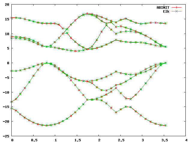
gnuplot> plot 'bands.dat' u 1:2 w lp title 'ABINIT', 'bands.dat' u 1:3 w lp title 'Elk'
You should get a graph like this:
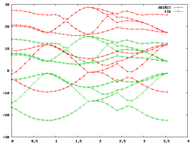
As you can see, the band structures look alike but differ by an absolute
shift, which is normal, because in a periodic system there is no unique vacuum
energy, and band energies are always defined up to an arbitrary constant
shift. This shift depends on the numerical details, and will be different for
different codes using different numerical approaches. (Note in the Elk input
file that the keyword xctype controls the type - LDA or GGA - of the
exchange-correlation functional.)
However, if we decide upon a reference pont, like the valence band maximum (VBM), or a point nearby, and align the two band plots at that point, there will still be differences. By comparing with the plot we just made, we see that the VBM is at the ninth k-point from the left, on band four. The script we used previously can accomodate a shift, by issuing the command:
python comp_bands_abinit2elk.py path/abinit_test/outputs/ab_C_test_o_DS42_EIG BAND.OUT align 9 4 eV
So that if the keyword align is present followed by the k-point index and
band number, we order the script to align at that point. Naturally, that will
make the positions of that particular point fit perfectly, but if we look at
the end of the output:
 ...
 # AVERAGES FOR OCCUPIED STATES:
 #        nvals:   106
 # average diff:     0.021871  eV
 # minimum diff:    -0.042755  eV
 # maximum diff:     0.064097  eV
 #
 # AVERAGES FOR UNOCCUPIED STATES:
 #        nvals:   174
 # average diff:     0.047221  eV
 # minimum diff:    -0.287747  eV
 # maximum diff:     0.089309  eV

 ...
we can tell that this is not true for the rest of the points. Since the script
assumes alignment at the VBM, it now separates its statistics for occupied and
unoccupied bands. The uppermost unoccupied bands can fit badly, depending on
what precision was asked of ABINIT (especially, if nbdbuf is used).
The fit is quite bad in general, an average of about 0.025 eV difference for
occupied states, and about 0.05 eV difference for unoccupied states. If you
plot the ouput as before, by piping the above to a bands.dat file and
executing the same gnuplot command, you should get the plot below.
On the scale of the band plot there is a small - but visible - difference between the two. Note that the deviations are usually larger away from the high-symmetry points, which is why it’s important to choose some points away from these as well when making these comparisons. However, it is difficult to conclude visually from the band structure that this is a bad dataset without using the statistics output by the script, and without some sense of what precision can be expected.
As we are now creating our “gold standard” with an Elk calculation, we also
need to calculate the equilibrium lattice parameter and Bulk modulus of
diamond with the Elk code. Unfortunately, Elk does not use datasets, so the
various lattice parameters we used in our ABINIT structural search will have
to be put in one by one by hand and the code run for each. The lattice
parameters in the ABINIT run were from 6.1 to 7.0 in increments of 0.1, so
that makes ten runs in total. To perform the first, simply edit the elk.in
file and change the keyword (at line 57):
 ...
 scale
 6.7403 : lattice parameter in Bohr
 ...
to:
 ...
 scale
 6.1 : lattice parameter in Bohr
 ...
Note
You also have to change the keyword frozencr to “.false.” because, at
the time of writing, there is an error in the calculation of the total energy
for frozen core-states. This means that the Elk input file must have the keyword (at line 65 ):
...
frozencr
.false.
...
Finally, you don’t need to calculate the band structure for each run, so you
might wand to change the tasks keyword section (at line 7):
 ...
 tasks
  0
  20
 ...
to just
 ...
 tasks
  0
 ...
After you’ve done these modifications, run Elk again. After the run has
finished, look in the TOTENERGY.OUT and the LATTICE.OUT files to get the
converged total energy and the volume. Write these down or save them in a safe
place, edit the elk.in file again, and so forth until you’ve calculated all
ten energies corresponding to the ten lattice parameter values. In the end you
should get a list which you can put in an eos.in file:
 "C - Diamond (Elk)"          : cname - name of material
 2                            : natoms - number of atoms
 1                            : etype - equation of state fit type
 50.0 95.0 100                : vplt1, vplt2, nvplt - start, end and #pts for fit
 10                           : nevpt - number of supplied points
 56.74525000  -75.5758514889
 59.58200000  -75.5933438506
 62.51175000  -75.6067015802
 65.53600000  -75.6163263051
 68.65625000  -75.6226219775
 71.87400000  -75.6259766731
 75.19075000  -75.6266976640
 78.60800000  -75.6250734731
 82.12725000  -75.6213749855
 85.75000000  -75.6158453243
(Your values might be slightly different in the last few decimals depending on
your system.) By running the eos utility as before we get:
 V0                =            74.47144624
 B0 (GPa)          =            469.7040543

 alatt = (4*74.47144624)^(1/3) = 6.6785 Bohr (3.5341 Å)
So we see that the initial, primitive, ABINIT dataset is about 9 GPa off for
the Bulk modulus and about 0.035 Bohr away from the correct value for the
lattice parameter. In principle, these should be about an order of magnitude
better, so let us see if we can make it so.
3.4. Carbon - improving the dataset
Now that you know the target values, is up to you to experiment and see if you can improve this dataset. The techniques are well documented in tutorial PAW2. Here’s a brief summary of main points to be concerned about:
- Use the keyword series
custom rrkj ..., orcustom polynom ..., orcustom polynom2 ..., if you want to have maximum control over the convergence properties of the projectors. - Check the logarithmic derivatives very carefully for the presence of ghost states.
- A dataset intended for ground-state calculations needs, as a rule of thumb, at least two projectors
per angular momentum channel. This is because only the occupied states need to be reproduced very accurately.
If you need to perform calculations which involve the Fock operator or unoccupied states
- like in GW calculations for instance - you will probably need at least three projectors. You might also want to add extra projectors in completely unoccupied \(l\)-channels.
We will now benchmark a more optimized atomic dataset for carbon. Try and check the convergence properties, equilibrium lattice parameter, bulk modulus, and bands for the input file below:
 C 6                                     ! Atomic name and number
 LDA-PW scalarrelativistic loggrid 801 logderivrange -10 40 1000 ! XC approx., SE type, gridtype, # pts, logderiv
 2 2 0 0 0 0                             ! maximum n for each l: 2s,2p,0d,0f..
 2 1 2                                   ! Partially filled shell: 2p^2
 0 0 0                                   ! Stop marker
 c                                       ! 1s - core
 v                                       ! 2s - valence
 v                                       ! 2p - valence
 1                                       ! l_max treated = 1
 1.3                                     ! core radius r_c
 y                                       ! Add unocc. s-state
 12.2                                    !  reference energy
 n                                       ! no more unoccupied s-states
 y                                       ! Add unocc. p-state
 6.9                                     !  reference energy
 n                                       ! no more unoccupied p-states
 custom polynom2 7 11 vanderbiltortho sinc   ! more complicated scheme for projectors
 3 0 ultrasoft                           ! localisation scheme
 1.3                                     ! Core radius for occ. 2s state
 1.3                                     ! Core radius for unoocc. 2s state
 1.3                                     ! Core radius for occ. 2p state
 1.3                                     ! Core radius for unocc. 2p state
 XMLOUT                                       ! Run atompaw2abinit converter
 prtcorewf noxcnhat nospline noptim      ! `ABINIT` conversion options
 0                                       ! Stop marker
Generate an atomic data file from this (you can replace the items in the old
input file if you want, or make a new directory for this study). You might
want to try and modify the gnuplot scripts so that they work correctly for
this dataset. (The wfn* files are ordered just like the core radius list at
the end, so now their meaning and the numbering of some other files have
changed.) There is an example of the modifications in the plot script
plot_C_all_II.p, which you
can download and run in gnuplot. You should get a plot like this:
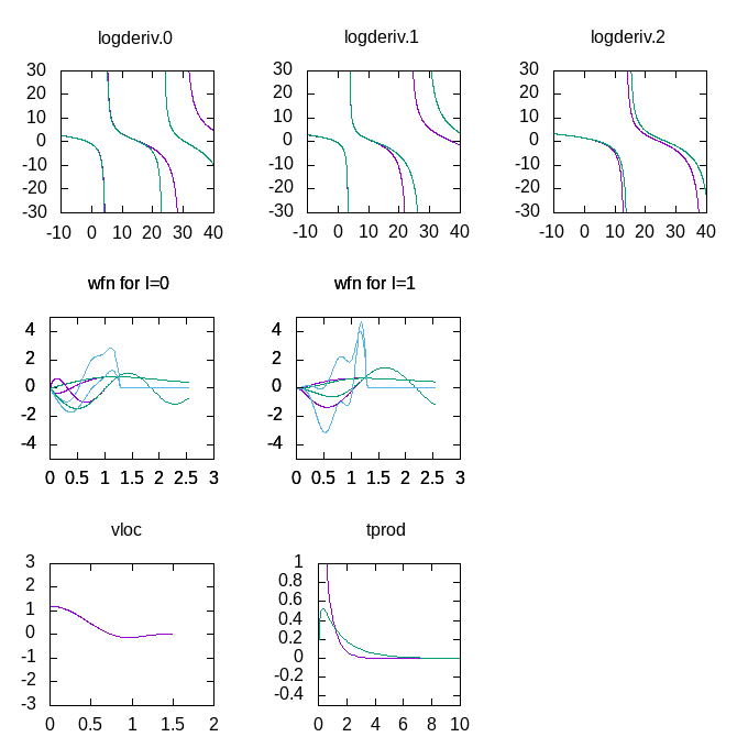
Note the much better fit of the logarithmic derivatives, and the change in the
shape of the projector functions (in blue in the wfn plots), due to the more
complicated scheme used to optimise them.
Generate the dataset like before and run the ABINIT ecut testing datasets in
the ab_C_test.abi ABINIT input file again. You should get an etotal
convergence like this (again, the values to the left are just there to help):
                                   etotal   (ecut)
  etotal11 -1.0785137440E+01
  etotal21 -1.1489028406E+01   - 703.89 mHa (10 Ha)
  etotal31 -1.1522398057E+01   -  33.37 mHa (15 Ha)
  etotal41 -1.1523369210E+01   -   0.97 mHa (20 Ha)
  etotal51 -1.1523467540E+01   -   0.10 mHa (25 Ha)
  etotal61 -1.1523515348E+01   -   0.05 mHa (30 Ha)
  etotal71 -1.1523525440E+01   -   0.01 mHa (35 Ha)
  etotal81 -1.1523552361E+01   -   0.03 mHa (40 Ha)
  etotal91 -1.1523572404E+01   -   0.02 mHa (45 Ha)
This dataset already seems to be converged to about 1 mHa at an ecut of 15 Ha,
so it is much more efficient. A comparison of bands (in units of eV) between
datasets 32 and 92 gives:
 ...
 #        nvals:   280
 # average diff:     0.004312  eV
 # minimum diff:    -0.013878  eV
 # maximum diff:     0.000544  eV
 ...
Which also shows a much faster convergence than before. Is the dataset
accurate enough? Well, if you run the ABINIT equilibrium parameter input file
in ab_C_equi.abi, you should get data for an eos.in file:
 "C - Diamond (second PAW dataset)" : cname - name of material
 2                                  : natoms - number of atoms
 1                                  : etype - equation of state fit type
 50.0 95.0 100                      : vplt1, vplt2, nvplt - start, end and #pts for fit
 10                                 : nevpt - number of supplied points
 5.6745250E+01  -1.1471957529E+01
 5.9582000E+01  -1.1489599125E+01
 6.2511750E+01  -1.1503102315E+01
 6.5536000E+01  -1.1512899444E+01
 6.8656250E+01  -1.1519381720E+01
 7.1874000E+01  -1.1522903996E+01
 7.5190750E+01  -1.1523789014E+01
 7.8608000E+01  -1.1522330567E+01
 8.2127250E+01  -1.1518796247E+01
 8.5750000E+01  -1.1513430193E+01
And when fed to eos, this gives us the equilibrium data:
 V0                =            74.71100799
 B0 (GPa)          =            465.7949258

 alatt = (4*74.71100799)^(1/3) = 6.6857 Bohr (3.5379 Å)
For comparison, we list all previous values again:
 Equilibrium        Bulk modulus       lattice
 volume, V0         B0                parameter
 75.5073            460.37            3.5505 Å   (1st primitive PAW dataset)
 74.7110            465.79            3.5379 Å   (2nd better PAW dataset)
 74.4714            469.70            3.5341 Å   (Elk all-electron)
It is obvious that the second dataset is much better than the first one. A comparison of the most converged values for the bands using the command:
python comp_bands_abinit2elk.py ab_C_test_o_DS92_EIG BAND.OUT align 9 4 eV
(This assumes that you have all the files you need in the current directory.) As before, the extra command parameters on the end mean “align the 9-th k-point on the fourth band and convert values to eV”. This will align the band structures at the valence band maximum. The statistics printed out at the end should be something like this:
 ...
 # AVERAGES FOR OCCUPIED STATES:
 #        nvals:   106
 # average diff:     0.013523  eV
 # minimum diff:    -0.001229  eV
 # maximum diff:     0.040695  eV
 #
 # AVERAGES FOR UNOCCUPIED STATES:
 #        nvals:   174
 # average diff:     0.016247  eV
 # minimum diff:    -0.013699  eV
 # maximum diff:     0.117064  eV
 ...
Which shows a precision, on average, of slightly better than 0.01 eV for both the four occupied and the four lowest unoccupied bands. As before, you can pipe this output to a file and plot the bands for visual inspection.
This is a better dataset, but probably by no means the best possible. It is likely that one can construct a dataset for carbon that has even better convergence properties, and is even more accurate. You are encouraged to experiment and try to make a better one.
4. Magnesium - dealing with the Fermi energy of a metallic system
There is added complication if the system is metallic, and that is the treatment of the smearing used in order to eliminated the sharp peaks in the density of states (DOS) near the Fermi energy. The DOS is technically integrated over in any ground-state calculation, and for a metal this requires, in principle, an infinite k-point grid in order to resolve the Fermi surface.
In practice, a smearing function is used so that a usually quite large - but finite - number of k-points will be sufficient. This smearing function has a certain spread controlled by a smearing parameter, and the optimum value of this parameter depends on the k-point grid used. As the k-point grid becomes denser, the optimum spread becomes smaller, and all values converge toward their ideal counterparts in the limit of no smearing and an infinitely dense grid.
The problem is that, in ABINIT, finding the optimum smearing parameter takes a
(potentially time consuming) convergence study. However, we are in luck. The
Elk code has an option for automatically determining the smearing parameter.
Thus we should use the Elk code first, set a relatively dense k-mesh, and
calculate the equilibrium bulk modulus, lattice parameter and band structure.
Then we make sure to match the automatically determined smearing width, and
most importantly, make sure that we match the smearing function used between
the Elk and the ABINIT calculation.
4.1. Magnesium - The all-electron calculation
There is an Elk input file prepared at: elk_Mg_band.in,
we suggest you copy it into a subdirectory dedicated to the Mg Elk calculation (why not Mg_elk?), rename
it to elk.in and take a look inside the input file.
! Carbon, diamond structure (FCC)

! The tasks define what will be done by the code:
! 0 - Perform ground-state calculation from scratch
! 1 - Restart GS calc. from STATE.OUT file
! 20 - Calculate band structure as defined by plot1d
tasks
1
20

ecvcut
 -6.0

species
 12 : atomic number
 'Mg'
 'magnesium'
 44305.30461        : atomic mass
 1.899259351   37.6052   : muffin-tin radius
   5                : number of occ. states
   1   0   1   2    : 1s
   2   0   1   2    : 2s
   2   1   1   2    : 2p m=0
   2   1   2   4    : 2p m=1
   3   0   1   2    : 3s
!  -6.0              : core-valence cutoff energy

! Tolerance on convegence of band energies (absolute)
epsband
 1.e-8

! Tolerance on conv. of potential (relative)
epspot
 1.e-7

! Tolerance on conv. of total energy (absolute)
epsengy
 1.e-6

! Use adaptive linear mixing of densities
! 1 - Adaptive linear
! 2 - Pulay mixing
mixtype
 3

! Exchange-correlation functional to use
! LDA (PW92) is 3 (default) (equiv. Abinit ixc 7)
! GGA-PBE    is 20          (equiv. Abinit ixc 11)
! (see Elk manual for other options)
xctype
 3

! Define lattice vectors
! Magnesium has a hexagonal native structure
! with a=b=3.20927 Å c=5.21033 Å  alpha=90 beta=90 gamma=60

! Scale factor to be applied to all lattice vectors
scale
 1.00

avec
     6.0646414   0.0000000   0.0000000
     3.0323207   5.2521335   0.0000000
     0.0000000   0.0000000   9.8460968

! Define atomic species
atoms
   1   : nspecies - Number of species
'Mg.in' : spfname - Name of species file
   2   : natoms; atposl, bfcmt below - Atoms in cell, reduced coord. and moments
    0.33333333    0.33333333    0.2500000    0.00000000  0.00000000  0.00000000
    0.66666666    0.66666666    0.7500000    0.00000000  0.00000000  0.00000000

! Don't set muffin-tin radius automatically
autormt
 .false.

! Freeze core states (in abinit PAW, they are frozen)
frozencr
 .true.

! Path to atomic data files
sppath
  './'

! Monkhorst-pack k-point grid
ngridk
 10  10  10

! Shift of MP grid
vkloff
0.0 0.0 0.5

! Metallic options
stype
 0          : Smearing type 0 - Gaussian
autoswidth
 .true.     : Automatic determination of swidth

! Set upper limit of |G+k|, the number below is
! (MT radius)*max(|G+k|)
rgkmax
9.0

! A value of 0.0 makes this being set automatically
gmaxvr
0.0

! k-points in band plot
plot1d
47 47  : nvp1d, npp1d
                     0.00000000E+00  0.00000000E+00  5.00000000E-01
                     8.33333333E-02  0.00000000E+00  5.00000000E-01
                     1.66666667E-01  0.00000000E+00  5.00000000E-01
                     2.50000000E-01  0.00000000E+00  5.00000000E-01
                     3.33333333E-01  0.00000000E+00  5.00000000E-01
                     4.16666667E-01  0.00000000E+00  5.00000000E-01
                     5.00000000E-01  0.00000000E+00  5.00000000E-01
                     4.72222222E-01  5.55555556E-02  5.00000000E-01
                     4.44444444E-01  1.11111111E-01  5.00000000E-01
                     4.16666667E-01  1.66666667E-01  5.00000000E-01
                     3.88888889E-01  2.22222222E-01  5.00000000E-01
                     3.61111111E-01  2.77777778E-01  5.00000000E-01
                     3.33333333E-01  3.33333333E-01  5.00000000E-01
                     2.77777778E-01  2.77777778E-01  5.00000000E-01
                     2.22222222E-01  2.22222222E-01  5.00000000E-01
                     1.66666667E-01  1.66666667E-01  5.00000000E-01
                     1.11111111E-01  1.11111111E-01  5.00000000E-01
                     5.55555556E-02  5.55555556E-02  5.00000000E-01
                     0.00000000E+00  0.00000000E+00  5.00000000E-01
                     0.00000000E+00  0.00000000E+00  4.50000000E-01
                     0.00000000E+00  0.00000000E+00  4.00000000E-01
                     0.00000000E+00  0.00000000E+00  3.50000000E-01
                     0.00000000E+00  0.00000000E+00  3.00000000E-01
                     0.00000000E+00  0.00000000E+00  2.50000000E-01
                     0.00000000E+00  0.00000000E+00  2.00000000E-01
                     0.00000000E+00  0.00000000E+00  1.50000000E-01
                     0.00000000E+00  0.00000000E+00  1.00000000E-01
                     0.00000000E+00  0.00000000E+00  5.00000000E-02
                     0.00000000E+00  0.00000000E+00  0.00000000E+00
                     8.33333333E-02  0.00000000E+00  0.00000000E+00
                     1.66666667E-01  0.00000000E+00  0.00000000E+00
                     2.50000000E-01  0.00000000E+00  0.00000000E+00
                     3.33333333E-01  0.00000000E+00  0.00000000E+00
                     4.16666667E-01  0.00000000E+00  0.00000000E+00
                     5.00000000E-01  0.00000000E+00  0.00000000E+00
                     4.72222222E-01  5.55555556E-02  0.00000000E+00
                     4.44444444E-01  1.11111111E-01  0.00000000E+00
                     4.16666667E-01  1.66666667E-01  0.00000000E+00
                     3.88888889E-01  2.22222222E-01  0.00000000E+00
                     3.61111111E-01  2.77777778E-01  0.00000000E+00
                     3.33333333E-01  3.33333333E-01  0.00000000E+00
                     2.77777778E-01  2.77777778E-01  0.00000000E+00
                     2.22222222E-01  2.22222222E-01  0.00000000E+00
                     1.66666667E-01  1.66666667E-01  0.00000000E+00
                     1.11111111E-01  1.11111111E-01  0.00000000E+00
                     5.55555556E-02  5.55555556E-02  0.00000000E+00
                     0.00000000E+00  0.00000000E+00  0.00000000E+00

! Number of empty bands to include
nempty
10

! Ratio betwen fine and coarse radial grid
! (the coarse grid is used for the calcualation
!  of densities). This needs to be set to one
! so that the grid specified in the .in file
! of the atomic species is used everywhere
lradstp
 1       : coarse/fine radial grid ratio
There will be sections familiar from before, defining the lattice vectors, structure, etc. (Mg has a 2-atom hexagonal unit cell.) Then there are a couple of new lines for the metallic case:
 ...
 ! Metallic options
 stype
  0          : Smearing type 0 - Gaussian
 autoswidth
  .true.     : Automatic determination of swidth
 ...
When you run Elk with this file, it will start a ground-state run (this might
take some time due to the dense k-point mesh), all the while automatically
determining the smearing width. At the end of the calculation the final value
of swidth will have been determined, and can be easily extracted with a grep:
grep ' smearing' INFO.OUT
this should furnish you with a list:
 Automatic determination of smearing width
 New smearing width :   0.1000000000E-02
 New smearing width :   0.4116175210E-02
 New smearing width :   0.4056329377E-02
 New smearing width :   0.4060342507E-02
 New smearing width :   0.4078123678E-02
 New smearing width :   0.4097424577E-02
 New smearing width :   0.4105841081E-02
 New smearing width :   0.4109614663E-02
 New smearing width :   0.4109651379E-02
 New smearing width :   0.4109804149E-02
 New smearing width :   0.4109807004E-02
 New smearing width :   0.4109805701E-02
 New smearing width :   0.4109804616E-02
 New smearing width :   0.4109804468E-02
 New smearing width :   0.4109804441E-02
 New smearing width :   0.4109804423E-02
where the last value is the one we seek, i.e. the smearing at convergence.
Since this Elk file will also calculate the band structure, you will have a
BAND.OUT file at the end of this calculation to compare your ABINIT band
structure to. There is one more thing we need to check, and that is the Fermi energy:
 grep 'Fermi  ' INFO.OUT

 Fermi                       :     0.116185305134
 Fermi                       :     0.115496524671
 Fermi                       :     0.122186414492
 Fermi                       :     0.128341839155
 Fermi                       :     0.132281493053
 Fermi                       :     0.133819140456
 Fermi                       :     0.134308473303
 Fermi                       :     0.134328785350
 Fermi                       :     0.134347853104
 Fermi                       :     0.134347939064
 Fermi                       :     0.134347635069
 Fermi                       :     0.134347477436
 Fermi                       :     0.134347453635
 Fermi                       :     0.134347448126
 Fermi                       :     0.134347446032
 Fermi                       :     0.134347446149
The last one is the Fermi energy at convergence. We will need this later when we compare band structures to align the band plots at the Fermi energy.
Now it’s time to calculate the equilibrium lattice parameters. There is a prepared file at: elk_Mg_equi.in.
! Carbon, diamond structure (FCC)

! The tasks define what will be done by the code:
! 0 - Perform ground-state calculation from scratch
! 1 - Restart GS calc. from STATE.OUT file
! 20 - Calculate band structure as defined by plot1d
tasks
0

!species
! 12 : atomic number
! 'Mg'
! 'magnesium'
! 44305.30461        : atomic mass
! 1.899259351   37.6052   : muffin-tin radius
!   5                : number of occ. states
!   1   0   1   2    : 1s
!   2   0   1   2    : 2s
!   2   1   1   2    : 2p m=0
!   2   1   2   4    : 2p m=1
!   3   0   1   2    : 3s
!  -6.0              : core-valence cutoff energy

! Tolerance on convegence of band energies (absolute)
epsband
 1.e-8

! Tolerance on conv. of potential (relative)
epspot
 1.e-7

! Tolerance on conv. of total energy (absolute)
epsengy
 1.e-6

! Use adaptive linear mixing of densities
! 1 - Adaptive linear
! 2 - Pulay mixing
mixtype
 3

! Exchange-correlation functional to use
! LDA (PW92) is 3 (default) (equiv. Abinit ixc 7)
! GGA-PBE    is 20          (equiv. Abinit ixc 11)
! (see Elk manual for other options)
xctype
 3

! Define lattice vectors
! Magnesium has a hexagonal native structure
! with a=b=3.20927 Å c=5.21033 Å  alpha=90 beta=90 gamma=60
! (experimental, at 25 degrees Celsius)

! Scale factor to be applied to all lattice vectors
scale
 1.00

avec
     6.0646414   0.0000000   0.0000000
     3.0323207   5.2521335   0.0000000
     0.0000000   0.0000000   9.8460968

! Define atomic species
atoms
   1   : nspecies - Number of species
'Mg.in' : spfname - Name of species file
   2   : natoms; atposl, bfcmt below - Atoms in cell, reduced coord. and moments
    0.33333333    0.33333333    0.2500000    0.00000000  0.00000000  0.00000000
    0.66666666    0.66666666    0.7500000    0.00000000  0.00000000  0.00000000

! Don't set muffin-tin radius automatically
autormt
 .false.

! Freeze core states (in abinit PAW, they are frozen)
frozencr
 .false.

! Path to atomic data files
sppath
  './'

! Monkhorst-pack k-point grid
ngridk
 10  10  10

! Shift of MP grid
vkloff
0.0 0.0 0.5

! Metallic options
stype
 0          : Smearing type 0 - Gaussian
swidth
 0.4109804423E-02      : Smearing width

! Set upper limit of |G+k|, the number below is
! (MT radius)*max(|G+k|)
rgkmax
9.0

! A value of 0.0 makes this being set automatically
gmaxvr
0.0

! Number of empty bands to include
nempty
10

! Ratio betwen fine and coarse radial grid
! (the coarse grid is used for the calcualation
!  of densities). This needs to be set to one
! so that the grid specified in the .in file
! of the atomic species is used everywhere
lradstp
 1       : coarse/fine radial grid ratio
As before copy this to your directory rename it to elk.in. The layout of this file looks pretty much
like the one before, except the band structure keywords are missing, and now
switdth is fixed to the value we extracted before:
 ...
 ! Metallic options
 stype
  0          : Smearing type 0 - Gaussian
 swidth
  0.4109804423E-02     : Smearing width
 ...
To calculate the equilibrium lattice parameters, we are going to use the bulk
modulus, which is a quantity defined with respect to a scaling of the entire
cell (as opposed to Young’s modulus, for instance, which is defined with
respect to linear scaling along the lattice vectors). There is a handy scale
keyword for Elk, which will accomplish this for us. If we look at the region
where the lattice is defined:
 ...
 ! Define lattice vectors
 ! Magnesium has an hexagonal native structure
 ! with a=b=3.20927 Å c=5.21033 Å  alpha=90 beta=90 gamma=60
 ! (experimental, at 25 degrees Celsius)

 ! Scale factor to be applied to all lattice vectors
 scale
  1.00

  with
       6.0646414   0.0000000   0.0000000
       3.0323207   5.2521335   0.0000000
       0.0000000   0.0000000   9.8460968
 ...
We will here also need to perform several calculations (like we did for the
diamond case) and we need to change the value of the scale keyword for each
one. A good set of values would be: 0.94, 0.96, 0.98, 1.0, 1.02 1.04 and 1.06,
i.e. a change of scale in steps of 2% with seven values in total spaced around
the experimental equilibrium lattice structure.
After each run, as before, you should collect the value of the unit cell
volume and the total energy. After seven runs you should have a set of numbers
which you can put in an eos.in file (depending on the system, your actual
values may differ slightly from these):
 "Mg - bulk metallic"
  2                      : natoms - number of atoms
  1                      : etype - equation of state fit type
  260.0 374.0 100        : vplt1, vplt2, nvplt - start, end and #pts for fit
  7                      : nevpt - number of supplied points
  260.4884939  -399.042203252
  277.4716924  -399.044435776
  295.1774734  -399.044943459
  313.6208908  -399.043962316
  332.8169982  -399.041812744
  352.7808497  -399.038751783
  373.5274988  -399.034932869
Upon using the eos utility you will get standard type of outputs in PARAM.OUT:
 Mg - bulk metallic

 Universal EOS
 Vinet P et al., J. Phys.: Condens. Matter 1, p1941 (1989)

 (Default units are atomic: Hartree, Bohr etc.)

  V0                =            291.6029247
  E0                =           -399.0449584
  B0                =           0.1364455738E-02
  B0'               =            4.304295809

  B0 (GPa)          =            40.14366703
Now we have to translate this in terms of the lattice parameters. The equilibrium scale factor is given by: \(scale = (\frac{V_0}{V_1})^{\frac{1}{3}} = (\frac{291.6029247}{313.6208908})^{\frac{1}{3}} = 0.9760280459\)
Where \(V_1\) is the volume with scale set to 1.0. Multiplying all basis vectors with this scale factor, we have that:
 Equilibrium        Bulk modulus       lattice
 volume, V0         B0                parameters
 291.6029           40.1437            a = b = 3.1323 Å  c = 5.0854 Å
Now we have all the information needed to proceed with the ABINIT calculation.
4.2. Magnesium - The ABINIT calculation
As usual, it’s best to prepare a separate subdirectory for the atomic data and
the ABINIT test. We will assume that the subdirectories have been created as:
 mkdir Mg_atompaw
 mkdir Mg_atompaw/abinit_test
 mkdir Mg_atompaw/abinit_test/outputs
and that your current directory is ./Mg_atompaw. For the Mg ATOMPAW input,
use the file Mg.input.
Mg 12
LDA-PW scalarrelativistic loggrid 801 40. logderivrange -10 40 1000
3 3 0 0 0 0
3 1 0
0 0 0
c
v
v
v
v
1
1.9
n
n
custom polynom2 7 11 vanderbiltortho sincshape
2 0 ultrasoft
1.9
1.9
1.9
1.9
XMLOUT
prtcorewf noxcnhat nospline noptim
END
Note that there are not really many projectors in this dataset, only two
per angular momentum channel. It should be possible to make this much better
adding extra projectors, and maybe even unoccupied \(d\)-states. If you run
atompaw with this, you can have a look with the bundled plot_MG_all.p file
and others like it to get a feel for the quality of this dataset.
Generate the ABINIT dataset file, and make sure it’s given as:
./Mg_atompaw/Mg_LDA-PW-paw.xml, then go to the subdirectory for the ABINIT test,
and copy these files to it: ab_Mg_test.abi,
and ab_Mg_equi.abi.
The file for testing the convergence has already been set up so that the smearing
strategy is equivalent to the Elk one, as evidenced by the lines:
# Input for PAW3 tutorial
# Mg - hexagonal structure

#-------------------------------------------------------------------------------
#Directories and files

pseudos="Mg.LDA-PW-paw.xml"

pp_dirpath="../"
outdata_prefix="outputs/ab_Mg_test_o"
tmpdata_prefix="outputs/ab_Mg_test"


#-------------------------------------------------------------------------------
#Define the different datasets

ndtset 18       # 18 double-index datasets
udtset 9 2      # 1st index running from 1 to 9 and the 2nd from 1 to 2

#Cutoff variables
ecut:?  5.0
ecut+?  5.0
pawecutdg 110.0
ecutsm 0.5

#Dataset 1
#Ground-state run
kptopt?1 1
nshiftk?1 1
shiftk?1 0.0 0.0 0.5
ngkpt 10 10 10
tolvrs?1 1.0d-14
nstep?1  150
getwfk21 11
getwfk31 21
getwfk41 31
getwfk51 41
getwfk61 51
getwfk71 61
getwfk81 71
getwfk91 81
nbdbuf?1 5
nband?1  25

#Dataset 2
#Definition of the k-point grid
#the band structure
iscf?2    -2
getden?2  -1
kptopt?2  -7
nband?2   20
nbdbuf?2   0
ndivk?2    6 6 6 10 6 6 6 # divisions of the 6 segments
kptbounds?2
           0   0   1/2 # A
           1/2 0   1/2 # L
           1/3 1/3 1/2 # H
           0   0   1/2 # A
           0   0   0   # Gamma
           1/2 0   0   # M
           1/3 1/3 0   # K
           0   0   0   # Gamma

tolwfr?2  1.0d-18
enunit?2  0             # Will output the eigenenergies in Ha
nstep?2   150


#-------------------------------------------------------------------------------
#Definition of the Unit cell

#Definition of the unit cell (hexagonal)
acell 2*3.20927 5.21033 angstrom
angdeg 90 90 60

#Definition of the atom types
ntypat 1          # One tom type
znucl 12           # Magnesium

#Definition of the atoms
natom 2           # 2 atoms per cell
typat 1 1         # each of type carbon
xred              # This keyword indicates that the location of the atoms
                  # will follow, one triplet of number for each atom
   1/3   1/3   1/4
   2/3   2/3   3/4

#Parameters for metals
tsmear 0.4109804423E-02
occopt 7

#-------------------------------------------------------------------------------
#Miscelaneous

#GS convergence fix
istwfk *1
# Input for PAW3 tutorial
# Mg - hexagonal structure - metallic bulk

#-------------------------------------------------------------------------------
#Directories and files

pseudos="Mg.LDA-PW-paw.xml"

pp_dirpath="../"
outdata_prefix="outputs/ab_Mg_equi_o"
tmpdata_prefix="outputs/ab_Mg_equi"


#-------------------------------------------------------------------------------
#Define the different datasets

ndtset 7             # 7 datasets
acell: 3*0.94 Bohr   # The starting values of the cell parameters
acell+ 3*0.02 Bohr   # The increment of acell from one dataset to the other


#-------------------------------------------------------------------------------
#Convergence parameters

#Cutoff variables
ecut  15.0
pawecutdg 110.0
ecutsm 0.5

#Definition of the k-point grid
chksymbreak 0
kptopt 1
nshiftk 1
shiftk 0.0 0.0 0.5
ngkpt 10 10 10

#Bands and occupations
nband  25
nbdbuf 5

#Parameters for metals
tsmear 0.4109804423E-02
occopt 7

#SCF cycle parameters
tolvrs 1.0d-14
nstep  150


#-------------------------------------------------------------------------------
#Definition of the Unit cell

#Definition of the unit cell
acell 3*1.
rprim
     6.0646414   0.0000000   0.0000000
     3.0323207   5.2521335   0.0000000
     0.0000000   0.0000000   9.8460968

#Definition of the atom types
ntypat 1          # One tom type
znucl 12          # Magnesium

#Definition of the atoms
natom 2           # 2 atoms per cell
typat 1 1         # each of type carbon
xred              # This keyword indicates that the location of the atoms
                  # will follow, one triplet of number for each atom
   1/3   1/3   1/4
   2/3   2/3   3/4
 ...
 # Parameters for metals
 tsmear 0.4109804423E-02
 occopt 7
 ...
inside it. The occopt 7 input variable corresponds exactly to the Gaussian
smearing which is the default for the Elk code. (In fact it is the 0th order
Methfessel-Paxton expression [Methfessel1989], for other
possibilities compare the entries for the keyword stype in the Elk manual
and the entries for occopt in ABINIT).
Now run the test input file (if your computer has several cores, you might
want to take advantage of that and run ABINIT in parallel). The test suite can
take some time to complete, because of the dense k-point mesh sampling. Make
sure you pipe the screen to a log file: log_Mg_test
When the run is finished, we can check the convergence properties as before,
and we that an ecut of 15 Ha is definitely enough. The interesting thing will
now be to compare the band structures. First we need to check the Fermi energy
of the ABINIT calculation, if you do a grep:
grep ' Fermi' log_Mg_test
you will see a long list of Fermi energies, one for each iteration, finally converging towards one number:
 ...
 newocc : new Fermi energy is       0.137605 , with nelect=     20.000000
 newocc : new Fermi energy is       0.137605 , with nelect=     20.000000
 newocc : new Fermi energy is       0.137605 , with nelect=     20.000000
The last one of these is the final Fermi energy of the ABINIT calculation. The
abinit2elk band comparison script can now be given the Fermi energies of the
two different calculations and align band structures there. Copy the
BAND.OUT file from the Elk calculation to the current directory, as well as
the band comparison script comp_bands_abinit2elk.py. This script can also be
used to align the bands at different Fermi energies. However, in the
BAND.OUT file from Elk, the bands are already shifted so that the Fermi
energy is at zero, so it is only the alignment of the ABINIT file that is required:
python comp_bands_abinit2elk.py ./outputs/ab_Mg_test_o_DS32_EIG BAND.OUT Fermi 0.137605 0.0 eV
Issuing this command will provide the final lines:
 ...
 #        nvals:   940
 # average diff:     0.029652  eV
 # minimum diff:    -0.036252  eV
 # maximum diff:     0.215973  eV
 ...
Which means that we are on average accurate to about 0.03 eV. If you pipe the
output to a file bands_abinit_elk.dat, and go into gnuplot and use the script plot_Mg_bands.p:
gnuplot> load 'plot_Mg_bands.p'
You should get a plot that looks something like this:
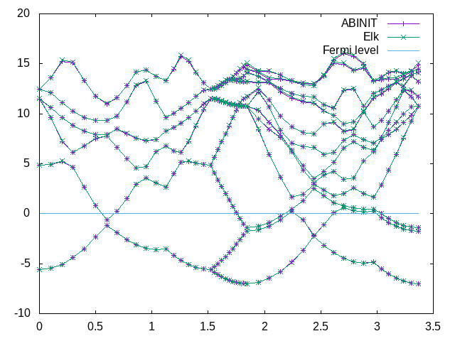
As we can see, the bands should fit quite well. Finally, for the structural, a
run of the ab_Mg_equi.abi file gives us all the information we need for the
creation of an eos.in file:
 "Mg - bulk metallic (ABINIT)"
  2                      : natoms - number of atoms
  1                      : etype - equation of state fit type
  260.0 380.0 100        : vplt1, vplt2, nvplt - start, end and #pts for fit
  7                      : nevpt - number of supplied points
  2.6048849E+02  -1.2697509579E+02
  2.7747169E+02  -1.2697742149E+02
  2.9517747E+02  -1.2697801365E+02
  3.1362089E+02  -1.2697716194E+02
  3.3281700E+02  -1.2697512888E+02
  3.5278085E+02  -1.2697212368E+02
  3.7352750E+02  -1.2696833809E+02
When the eos utility is run, we get the equilibrium volume and Bulk modulus:
 ...
 V0                =            293.0281803
 ...
 B0 (GPa)          =            39.19118222
Converting this to lattice parameters as before, we can compare this with the Elk run:
 Equilibrium        Bulk modulus       lattice
 volume, V0         B0                parameters
 291.6029           40.1437        a = b = 3.1323 Å  c = 5.0854 Å  (Elk)
 293.0282           39.1912        a = b = 3.1374 Å  c = 5.0937 Å  (ABINIT)
Which is very close.
Again, this is a decent dataset for ground-state calculations, but it can probably be made even better. You are encouraged to try and do this.
5. PAW datasets for GW calculations
There are a number of issues to consider when making datasets for GW calculations, here is a list of a few:
-
Care needs to be taken so that the logarithmic derivatives match for much higher energies than for ground-state calculations. They should at least match well up to the energy of the unoccupied states used in the calculation. The easiest way of ensuring this is increasing the number of projectors per state.
-
The on-site basis needs to be of higher quality to minimise truncation error due to the finite number of on-site basis functions (projectors). Again, this requires more projectors per angular momentum channel.
-
As a rule of thumb, a PAW dataset for GW should have at least three projectors per state, if not more.
-
A particularly sensitive thing is the quality of the expansion of the pseudised plane-wave part in terms of the on-site basis. This can be checked by using the density of states (DOS), as described in the first PAW tutorial.