Tutorial on DFT+DMFT

A DFT+DMFT calculation for SrVO₃.

This tutorial aims at showing how to perform a DFT+DMFT calculation using Abinit.

You will not learn here what is DFT+DMFT. But you will learn how to do a DFT+DMFT calculation and what are the main input variables controlling this type of calculation.

It might be useful that you already know how to do PAW calculations using ABINIT but it is not mandatory (you can follow the two tutorials on PAW in ABINIT, PAW1 and PAW2. Also the DFT+U tutorial in ABINIT might be useful to know some basic variables common to DFT+U and DFT+DMFT.

This tutorial should take about one hour to complete (less if you have access to several processors).

Note

Supposing you made your own installation of ABINIT, the input files to run the examples are in the ~abinit/tests/ directory where ~abinit is the absolute path of the abinit top-level directory. If you have NOT made your own install, ask your system administrator where to find the package, especially the executable and test files.

In case you work on your own PC or workstation, to make things easier, we suggest you define some handy environment variables by executing the following lines in the terminal:

export ABI_HOME=Replace_with_absolute_path_to_abinit_top_level_dir # Change this line
export PATH=$ABI_HOME/src/98_main/:$PATH      # Do not change this line: path to executable
export ABI_TESTS=$ABI_HOME/tests/             # Do not change this line: path to tests dir
export ABI_PSPDIR=$ABI_TESTS/Pspdir/  # Do not change this line: path to pseudos dir

Examples in this tutorial use these shell variables: copy and paste the code snippets into the terminal (remember to set ABI_HOME first!) or, alternatively, source the set_abienv.sh script located in the ~abinit directory:

source ~abinit/set_abienv.sh

The ‘export PATH’ line adds the directory containing the executables to your PATH so that you can invoke the code by simply typing abinit in the terminal instead of providing the absolute path.

To execute the tutorials, create a working directory (Work*) and copy there the input files of the lesson.

Most of the tutorials do not rely on parallelism (except specific tutorials on parallelism). However you can run most of the tutorial examples in parallel with MPI, see the topic on parallelism.

1 The DFT+DMFT method: summary and key parameters

The DFT+DMFT method aims at improving the description of strongly correlated systems. Generally, these highly correlated materials contain rare-earth metals or transition metals, which have partially filled d or f bands and thus localized electrons. For further information on this method, please refer to [Georges1996] and [Kotliar2006]. For an introduction to Many Body Physics (Green’s function, Self-energy, imaginary time, and Matsubara frequencies), see e.g. [Coleman2015] and [Tremblay2017].

Several parameters (both physical and technical) needs to be discussed for a DFT+DMFT calculation.

• The definition of correlated orbitals. In the ABINIT DMFT implementation, it is done with the help of Projected Wannier orbitals (see [Amadon2008]). The first part of the tutorial explains the importance of this choice. Wannier functions are unitarily related to a selected set of Kohn Sham (KS) wavefunctions, specified in ABINIT by band index dmftbandi, and dmftbandf. Thus, as empty bands are necessary to build Wannier functions, it is required in DMFT calculations that the KS Hamiltonian is correctly diagonalized: use high values for nnsclo, and nline for DMFT calculations and preceding DFT calculations. Roughly speaking, the larger dmftbandf-dmftbandi is, the more localized is the radial part of the orbital. Note that this definition is different from the definition of correlated orbitals in the DFT+U implementation in ABINIT (see [Amadon2008a]). The relation between the two expressions is briefly discussed in [Amadon2012].

• The definition of the Coulomb and exchange interaction U and J are done as in DFT+U through the variables upawu and jpawu. They could be computed with the cRPA method, also available in ABINIT. The value of U and J should in principle depend on the definition of correlated orbitals. In this tutorial, U and J will be seen as parameters, as in the DFT+U approach. As in DFT+U, two double counting methods are available (see the dmft_dc input variable).

• The choice of the double counting correction. The current default choice in ABINIT is (dmft_dc = 1) which corresponds to the full localized limit.

• The method of resolution of the Anderson model. In ABINIT, it can be the Hubbard I method (dmft_solv = 2) the Continuous time Quantum Monte Carlo (CTQMC) method (dmft_solv=5) or the static mean field method (dmft_solv = 1) equivalent to usual DFT+U.

• The solution of the Anderson Hamiltonian and the DMFT solution are strongly dependent over temperature. So the temperature tsmear is a very important physical parameter of the calculation.

• The practical solution of the DFT+DMFT scheme is usually presented as a double loop over first the local Green’s function, and second the electronic local density. (cf Fig. 1 in [Amadon2012]). The number of iterations of both loops are respectively given in ABINIT by keywords dmft_iter and nstep. Other useful variables are dmft_rslf = 1 and prtden = -1 (to be able to restart the calculation from the density file). Lastly, one linear and one logarithmic grid are used for Matsubara Frequencies indicated by dmft_nwli and dmft_nwlo (Typical values are 100000 and 100, but convergence should be studied). A large number of information are given in the log file using pawprtvol = 3.

2 Electronic Structure of SrVO3 in LDA

You might create a subdirectory of the *$ABI_TESTS/tutoparal directory, and use it for the tutorial. In what follows, the names of files will be mentioned as if you were in this subdirectory*

Copy the file tdmft_1.abi from $ABI_TESTS/tutoparal in your Work directory,

cd $ABI_TESTS/tutoparal/Input
mkdir Work_dmft
cd Work_dmft
cp ../tdmft_1.abi .

View tests/tutoparal/Input/tdmft_1.abi

Then run ABINIT with:

mpirun -n 24 abinit  tdmft_1.abi > log_1 &

This run should take some time. It is recommended that you use at least 10 processors (and 24 should be fast). It calculates the LDA ground state of SrVO3 and compute the band structure in a second step.

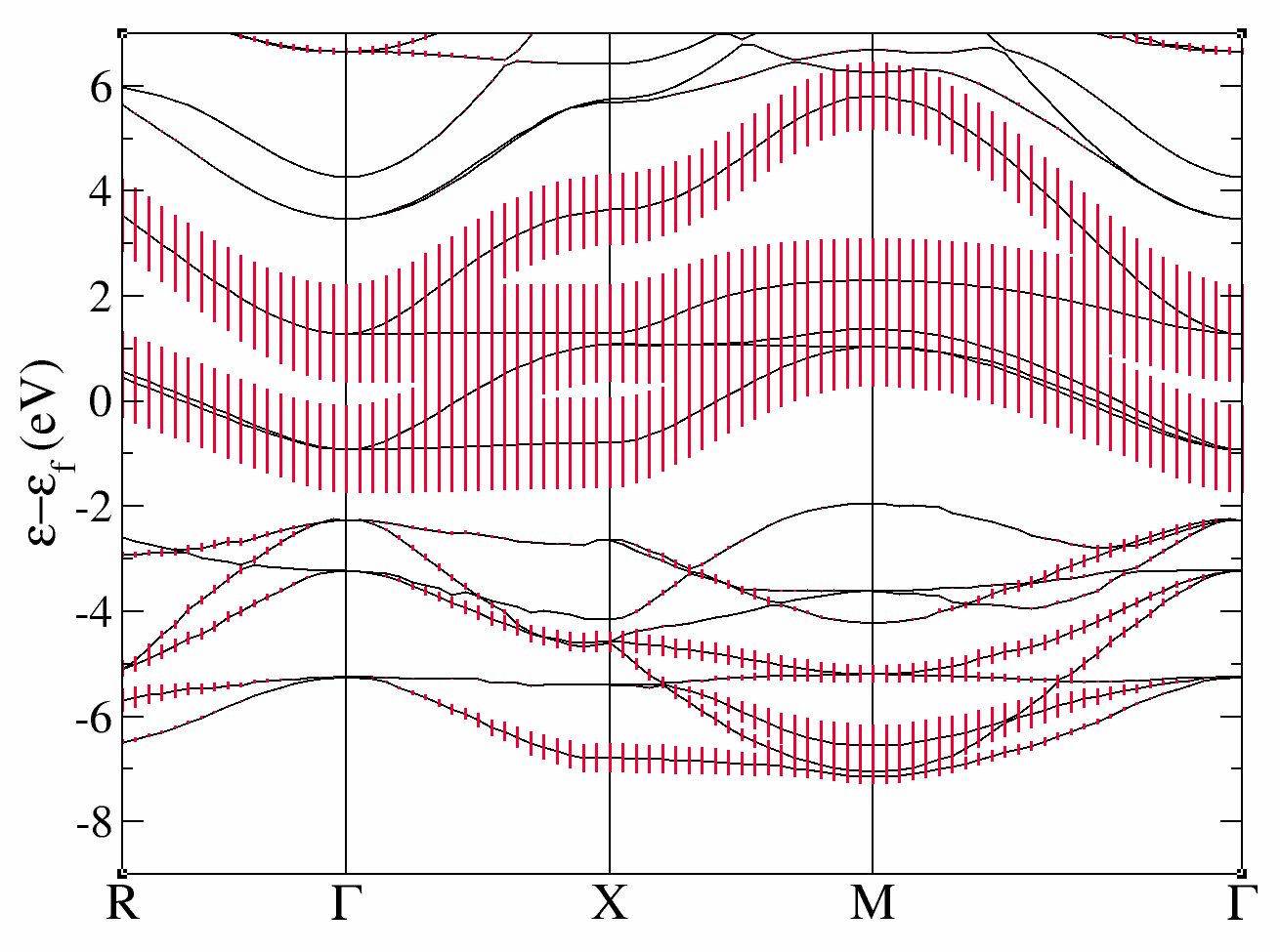
The variable pawfatbnd allows to create files with “fatbands” (see description of the variable in the list of variables): the width of the line along each k-point path and for each band is proportional to the contribution of a given atomic orbital on this particular Kohn Sham Wavefunction. A low cutoff and a small number of k-points are used in order to speed up the calculation.

During this time you can take a look at the input file. There are two datasets. The first one is a ground state calculations with nnsclo=3 and nline=3 in order to have well diagonalized eigenfunctions even for empty states. In practice, you have however to check that the residue of wavefunctions is small at the end of the calculation. In this calculation, we find 1.E-06, which is large (1.E-10 would be better, so nnsclo and nline should be increased, but it would take more time). When the calculation is finished, you can plot the fatbands for Vanadium and l=2. Several possibilities are available for that purpose. We will work with the simple xmgrace package (you need to install it, if not already available on your machine).

xmgrace tdmft_1o_DS2_FATBANDS_at0001_V_is1_l0002 -par ../Input/tdmft_fatband.par

The band structure is given in eV.

and the fatbands for all Oxygen atoms and l=1 with

xmgrace tdmft_1o_DS2_FATBANDS_at0003_O_is1_l0001 tdmft_1o_DS2_FATBANDS_at0004_O_is1_l0001 tdmft_1o_DS2_FATBANDS_at0005_O_is1_l0001 -par ../Input/tdmft_fatband.par

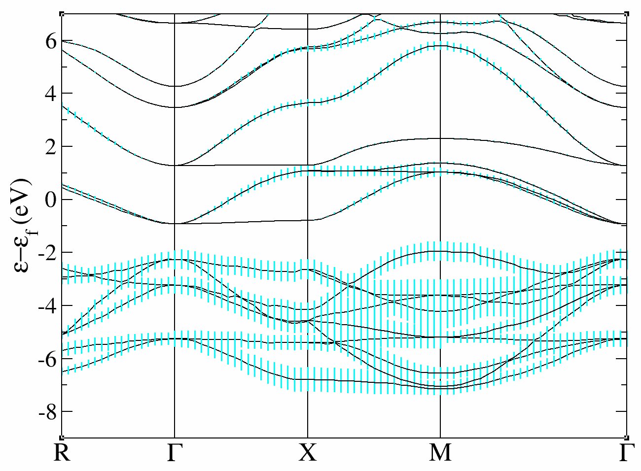
In these plots, you recover the band structure of SrVO3 (see for comparison the band structure of Fig.3 of [Amadon2008]), and the main character of the bands. Bands 21 to 25 are mainly d and bands 12 to 20 are mainly oxygen p. However, we clearly see an important hybridization. The Fermi level (at 0 eV) is in the middle of bands 21-23.

One can easily check that bands 21-23 are mainly d-t 2g and bands 24-25 are mainly e_g: just use pawfatbnd = 2 in tdmft_1.abi and relaunch the calculations. Then the file tdmft_1o_DS2_FATBANDS_at0001_V_is1_l2_m-2, tdmft_1o_DS2_FATBANDS_at0001_V_is1_l2_m-1 and tdmft_1o_DS2_FATBANDS_at0001_V_is1_l2_m1 give you respectively the xy, yz and xz fatbands (ie d-t 2g) and tdmft_1o_DS2_FATBANDS_at0001_V_is1_l2_m+0 and tdmft_1o_DS2_FATBANDS_at0001_V_is1_l2_m+2 give the z² and x²-y² fatbands (i.e. e_g).

So in conclusion of this study, the Kohn Sham bands which are mainly t_2g are the bands 21,22 and 23.

Of course, it could have been anticipated from classical crystal field theory: the vanadium is in the center of an octahedron of oxygen atoms, so d orbitals are split in t_2g and e_g. As t_2g orbitals are not directed toward oxygen atoms, t_2g-like bands are lower in energy and filled with one electron, whereas e_g-like bands are higher and empty.

In the next section, we will thus use the t_2g-like bands to built Wannier functions and do the DFT+DMFT calculation.

3 Electronic Structure of SrVO3: DFT+DMFT calculation

3.1. The input file for DMFT calculation: correlated orbitals, screened Coulomb interaction and frequency mesh

In ABINIT, correlated orbitals are defined using the projected local orbitals Wannier functions as outlined above. The definition requires to define a given energy window from which projected Wannier functions are constructed. We would like in this tutorial, to apply the DMFT method on d orbitals and for simplicity on a subset of d orbitals, namely t_2g orbitals ( e_g orbitals play a minor role because they are empty). But we need to define t_2g orbitals. For this, we will use Wannier functions.

As we have seen in the orbitally resolved fatbands, the Kohn Sham wave function contains a important weight of t_2g atomic orbitals mainly in t _2g-like bands but also in oxygen bands.

So, we can use only the t_2g-like bands to define Wannier functions or also both the t_2g-like and O-p -like bands.

The first case corresponds to the input file tdmft_2.abi. In this case dmftbandi = 21 and dmftbandf = 23. As we only put the electron interaction on t_2g orbitals, we have to use first lpawu = 2, but also the keyword dmft_t2g = 1 in order to restrict the application of interaction on t_2g orbitals.

Notice also that before launching a DMFT calculation, the LDA should be perfectly converged, including the empty states (check nline and nnsclo in the input file). The input file tdmft_2.abi thus contains two datasets: the first one is a well converged LDA calculation, and the second is the DFT+DMFT calculation.

Notice the other dmft variables used in the input file and check their meaning in the input variable glossary. In particular, we are using dmft_solv = 5 for the dmft dataset in order to use the density-density continuous time quantum monte carlo (CTQMC) solver. (See [Gull2011], as well as the ABINIT 2016 paper [Gonze2016] for details about the CTQMC implementation in ABINIT.) Note that the number of imaginary frequencies dmft_nwlo has to be set to at least twice the value of dmftqmc_l (the discretization in imaginary time). Here, we choose a temperature of 1200 K. For lower temperature, the number of Matsubara frequencies should be higher.

Here we use a fast calculation, with a small value of the parameters, especially dmft_nwlo, dmftqmc_l and dmftqmc_n.

Let’s now discuss the value of the effective Coulomb interaction U (upawu) and J (jpawu). The values of U and J used in ABINIT in DMFT use the same convention as in DFT+U calculations in ABINIT (cf [Amadon2008a]). However, calculations in Ref. [Amadon2008] use for U and J the usual convention for t_2g systems as found in [Lechermann2006], Eq. 26 (see also the appendix in [Fresard1997]). It corresponds to the Slater integral F4=0 and we can show that U_abinit=U-4/3 J and J_abinit=7/6 J. So in order to use U = 4 eV and J=0.65 eV with these latter conventions (as in [Amadon2008]), we have to use in ABINIT: upawu = 3.13333 eV; jpawu = 0.75833 eV and f4of2_sla = 0.

Now, you can launch the calculation:

Copy the file ../Input/tdmft_2.abi in your Work directory and run ABINIT:

mpirun -n 24 abinit tdmft_2.abi > log_2

View tests/tutoparal/Input/tdmft_2.abi

3.2. The DFT+DMFT calculation: the log file

We are now going to browse quickly the log file (log_2) for this calculation.

Starting from

=====  Start of DMFT calculation

we have first the definition of logarithmic grid for frequency, then, after:

== Prepare data for DMFT calculation

The projection of Kohn Sham wavefunctions and (truncated) atomic orbitals are computed (Eq.(2.1) in [Amadon2012]) and unnormalized orbitals are built (Eq.(2.2) in [Amadon2012]) The occupation matrix in this orbital basis is

  ------ Symetrised Occupation

        0.10480  -0.00000  -0.00000
        0.00000   0.10480  -0.00000
       -0.00000  -0.00000   0.10480

and the Normalization of this orbital basis is

  ------ Symetrised Norm

        0.62039   0.00000   0.00000
        0.00000   0.62039   0.00000
        0.00000   0.00000   0.62039

Now, let’s compare these numbers to other quantities. If the preceding LDA calculation is converged, dmatpuopt=1 is used, and dmftbandi=1 and dmftbandf=nband, then the above Symetrised Occupation should be exactly equal to the occupation matrix given in the usual DFT+U occupation matrix written in the log file (with dmatpuopt=1) (see discussion in [Amadon2012]). In our case, we are not in this case because dmftbandi=21 so this condition is not fulfilled. Concerning the norm if these orbitals, two factors play a role:

• Firstly, the number of Kohn Sham function used should be infinite (cf Eq. B.4 of [Amadon2012]), which is not the case here, because we take into account only bands 21-23. We emphasize that it is not a limitation of our approach, but just a physical choice concerning Wannier functions. This physical choice induces that these intermediate wave functions have a very low norm.

• Secondly, the atomic orbitals used to do the projection are cut at the PAW radius. As a consequence, even if we would use a complete set of KS wavefunctions and thus the closure relation, the norm could not be one. In our case, it could be at most 0.84179, which is the norm of the truncated atomic function of d orbitals of Vanadium used in this calculation. This number can be found in the log file by searching for ph0phiint (grep “ph0phiint(icount)= 1” log_2). (See also the discussion in Section B.3 of [Amadon2012]).

Next the LDA Green’s function is computed.

 =====  DFT Green Function Calculation

Then the Green’s function is integrated to compute the occupation matrix. Interestingly, the density matrix here must be equal to the density matrix computed with the unnormalized correlated orbitals. If this is not the case, it means that the frequency grid is not sufficiently large. In our case, we find:

        0.10481  -0.00000  -0.00000
       -0.00000   0.10481  -0.00000
       -0.00000  -0.00000   0.10481

So the error is very small (1.10E-5). As an exercise, you can decrease the number of frequencies and see that the error becomes larger.

Then the true orthonormal Wannier functions are built and the Green’s function is computed in this basis just after:

 =====  DFT Green Function Calculation with renormalized psichi

The occupation matrix is now:

        0.16893   0.00000  -0.00000
        0.00000   0.16893   0.00000
       -0.00000   0.00000   0.16893

We see that because of the orthonormalization of the orbitals necessary to built Wannier functions, the occupation matrix logically increases.

Then, after:

 =====  Define Interaction and self-energy

The Interaction kernel is computed from U and J, and the self energy is read from the disk file (if it exists). Then, the Green’s function is computed with the self energy and the Fermi level is computed. Then the DMFT Loop starts.

 =====  DMFT Loop starts here

The log contains a lot of details about the calculation (especially if pawprtvol=3). In order to have a more synthetic overview of the calculation (this is especially useful to detect possible divergence of the calculation), the following command extracts the evolution of the number of electrons (LDA, LDA with Wannier functions, and DMFT number of electrons) as a function of iterations (be careful, all numbers of electron are computed differently as explained in the log file):

grep -e Nb -e ITER log_2

Besides, during each DMFT calculation, there are one or more CTQMC calculations:

Starting QMC  (Thermalization)

For the sake of efficiency, the DMFT Loop is in this calculation done only once before doing again the DFT Loop (cf Fig. 1 of [Amadon2012]). At the end of the calculation, the occupation matrix is written and is:

          -- polarization spin component  1
        0.16811   0.00000  -0.00000
        0.00000   0.16811  -0.00000
       -0.00000  -0.00000   0.16811

We can see that the total number of electron is very close to one and it does not change much as a function of iterations. As an output of the calculation, you can find the self energy in file tdmft_2o_DS2Self-omega_iatom0001_isppol1 and the Green’s function is file Gtau.dat.

3.3. The self energy

You can use the self-energy to compute the quasiparticle renormalization weight. We first extract the first six Matsubara frequencies:

head -n 8 tdmft_2o_DS2Self-omega_iatom0001_isppol1 > self.dat

Then we plot the imaginary part of the self-energy (in imaginary frequency):

xmgrace -block self.dat -bxy 1:3

Then using xmgrace , you click on Data , then on Transformations and then on Regression and you can do a 4^th order fit as:

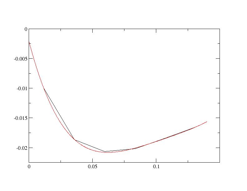
The slope at zero frequency obtained is 0.82. From this number, the quasiparticle renormalisation weight can be obtained using Z=1/(1+0.82)=0.55.

3.4. The Green’s function for correlated orbitals

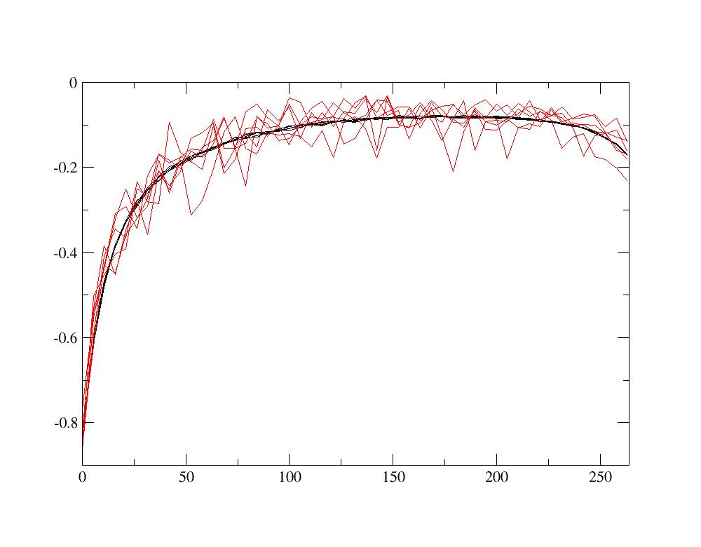
The impurity (or local) Green’s function for correlated orbitals is written in the file Gtau.dat. It is plotted as a function of the imaginary time in the interval [0, β] where β is the inverse temperature (in Hartree). You can plot this Green’s function for the six t_2g orbitals using e.g xmgrace

xmgrace -nxy Gtau.dat

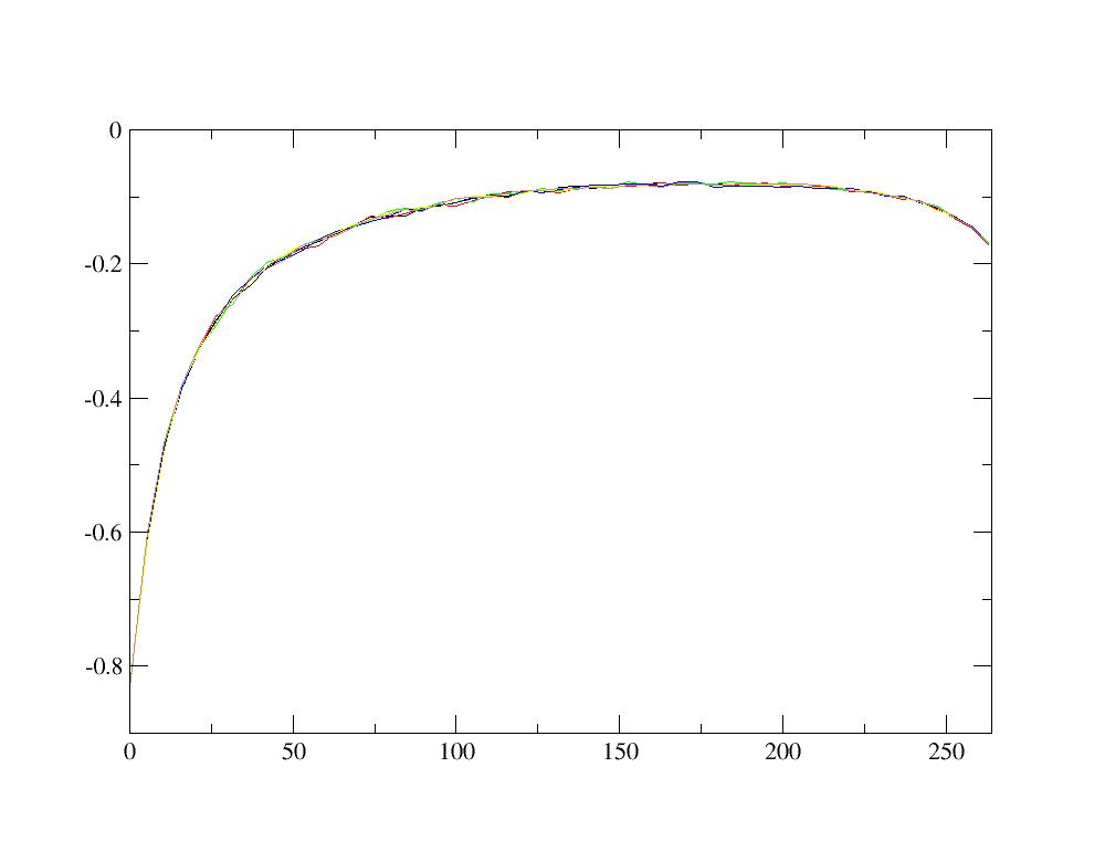
As the six _t 2g _ orbitals are degenerated, the six Green’s function must be similar, within the stochastic noise. Moreover, this imaginary time Green’s function must be negative and the value of G(β) for the orbital i is equal to the opposite of the number of electrons in the orbital i (-ni). Optionnally, you can check how the Green’s function can be a rough way to check for the importance of stochastic noise. For example, change for simplicity the number of steps for the DMFT calculation to 1:

nstep2 1

and then use a much smaller number of steps for the Monte Carlo Solver such as

dmftqmc_n 1.d3

save the previous Gtau.dat file:

cp Gtau.dat Gtau.dat_save

Then relaunch the calculation. After it is completed, compare the new Green’s function and the old one with the previous value of dmftqmc_n. Using xmgrace,

xmgrace -nxy Gtau.dat_save -nxy Gtau.dat

one obtains:

One naturally sees that the stochastic noise is much larger in this case. This stochastic noise can induces that the variation of physical quantities (number of electrons, electronic density, energy) as a function of the number of iteration is noisy. Once you have finished this comparison, copy the saved Green’s function into Gtau.dat in order to continue the tutorial with a precise Green’s function in Gtau.dat:

cp Gtau.dat_save Gtau.dat

3.5. The local spectral function

You can now use the imaginary time Green’s function (contained in file Gtau.dat) to compute the spectral function in real frequency. Such analytical continuation can be done on quantum Monte Carlo data using the Maximum Entropy method.

A maximum entropy code has been published recently by D. Bergeron. It can be downloaded here. Please cite the related paper [Bergeron2016] if you use this code in a publication.

The code has a lot of options, and definitely, the method should be understood and the user guide should be read before any real use. It is not the goal of this DFT+DMFT tutorial to introduce to the Maximum Entropy Method (see [Bergeron2016] and references therein). We give here a very quick way to obtain a spectral function. First, you have to install this code and the armadillo library by following the guidelines, and then launch it on the current directory in order to generate the default input file OmegaMaxEnt_input_params.dat.

OmegaMaxEnt

Then edit the file OmegaMaxEnt_input_params.dat, and modify the first seven lines with:

data file: Gtau.dat

OPTIONAL PREPROCESSING TIME PARAMETERS

DATA PARAMETERS
bosonic data (yes/[no]): no
imaginary time data (yes/[no]): yes

Then relaunch the code

OmegaMaxEnt

and plot the spectral function:

xmgrace OmegaMaxEnt_final_result/optimal_spectral_function_*.dat

Change the unit from Hartree to eV, and then, you have the spectral function:

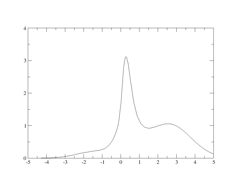
Even if the calculation is not well converged, you recognize in the spectral functions the quasiparticle peak as well as Hubbard bands at -2 eV and +2.5 eV as in Fig.4 of [Amadon2008].

4 Electronic Structure of SrVO3: Choice of correlated orbitals

Previously, only the t_2g-like bands were used in the definition of Wannier functions. If there were no hybridization between t_2g orbitals and oxygen p orbitals, the Wannier functions would be pure atomic orbitals and they would not change if the energy window was increased. But there is an important hybridization, as a consequence, we will now built Wannier functions with a large window, by including oxygen p -like bands in the definition of Wannier functions. Create a new input file:

cp tdmft_2.abi tdmft_3.abi

and use dmftbandi = 12 in tdmft_3.abi. Now the code will built Wannier functions with a larger window, including O-p -like bands, and thus much more localized. Launch the calculation (if the calculation is too long, you can decide to restart the second dataset directly from a converged LDA calculation instead of redoing the LDA calculation for each new DMFT calculation).

abinit tdmft_3.abi > log_3

In this case, both the occupation and the norm are larger because more states are taken into account: you have the occupation matrix which is

  ------ Symetrised Occupation

        0.22504  -0.00000  -0.00000
       -0.00000   0.22504  -0.00000
       -0.00000  -0.00000   0.22504

and the norm is:

  ------ Symetrised Norm

        0.73746   0.00000  -0.00000
        0.00000   0.73746  -0.00000
       -0.00000  -0.00000   0.73746

Let us now compare the total number of electron and the norm with the two energy window:

Energy window:	t2g-like bands	t2g-like+ O-p -like bands
dmftbandi/dmftbandf:	21/23	12/23
Norm:	0.63	0.78
LDA Number of electrons (before ⊥):	0.63(=0.105*6)	1.35(=0.235*6)
LDA Number of electrons (after ⊥):	1.00	1.77

For the large window, as we use more Kohn Sham states, both the occupation and the norm are larger, mainly because of the important weight of d orbitals in the oxygen bands (because of the hybridization). Concerning the norm, remind that in any case, it cannot be larger that 0.86. So as the Norm is 0.78, it means that by selecting bands 12-23 in the calculation, we took into account 0.78/0.86*100=90\% of the weight of the truncated atomic orbital among Kohn Sham bands. Moreover, after orthonormalization, you can check that the difference between LDA numbers of electrons is still large (1.02 versus 1.81), even if the orthonormalization effect is larger on the small windows case.

At the end of the DFT+DMFT calculation, the occupation matrix is written and is

          -- polarization spin component  1
        0.29313   0.00000   0.00000
        0.00000   0.29313   0.00000
        0.00000   0.00000   0.29313

Similarly to the previous calculation, the spectral function can be plotted using the Maximum Entropy code: we find a spectral function with an hybridation peak at -5 eV, as described in Fig.5 of [Amadon2008].

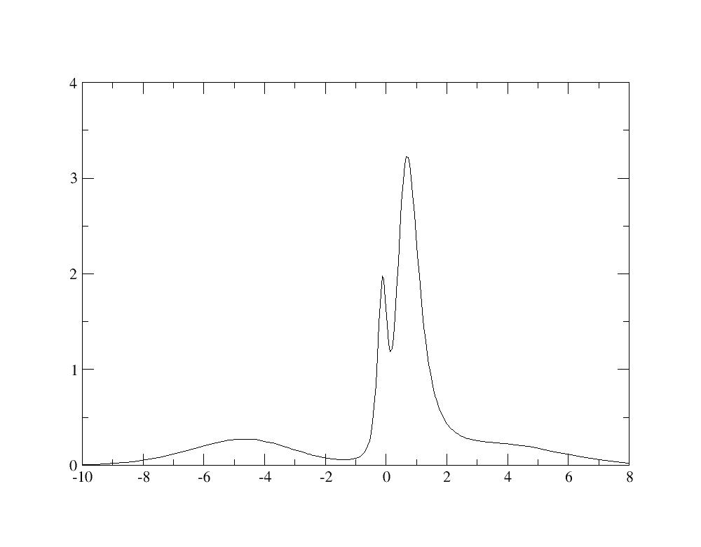
Resolving the lower Hubbard bands would require a more converged calculation.

As above, one can compute the renormalization weight and it gives 0.68. It shows that with the same value of U and J, interactions have a weaker effect for the large window Wannier functions. Indeed, the value of the screened interaction U should be larger because the Wannier functions are more localized (see discussion in [Amadon2008]).

5 Electronic Structure of SrVO3: The internal energy

The internal energy can be obtained with

grep -e ITER -e Internal log_3

and select the second occurrence for each iteration (the double counting expression) which should be accurate with iscf=17 (at convergence both expressions are equals also in DFT+DMFT). So after gathering the data:

Iteration	Internal Energy (Ha)
1	-1.51857850339126E+02
2	-1.51986727402835E+02
3	-1.51895311846530E+02
4	-1.51906820876597E+02
5	-1.51891956860157E+02
6	-1.51891135879190E+02
7	-1.51892587329592E+02
8	-1.51891607809905E+02
9	-1.51891447186423E+02
10	-1.51892343918492E+02

You can plot the evolution of the internal energy as a function of the iteration.

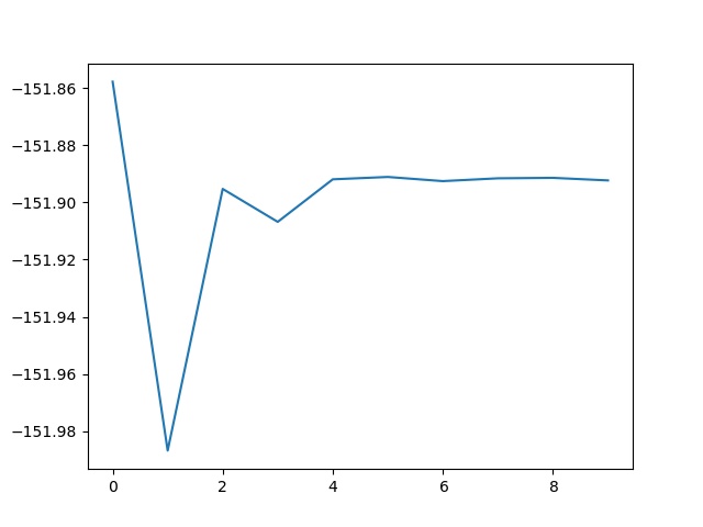
You notice that the internal energy (in a DFT+DMFT calculations) does not converge as a function of iterations, because there is a finite statistical noise. So, as a function of iterations, first, the internal energy starts to converge, because the modification of the energy induced by the self- consistency cycle is larger than the statistical noise, but then the internal energy fluctuates around a mean value. So if the statistical noise is larger than the tolerance, the calculation will never converge. So if a given precision on the total energy is expected, a practical solution is to increase the number of Quantum Monte Carlo steps (dmftqmc_n) in order to lower the statistical noise. Also another solution is to do an average over the last values of the internal energy.

6 Electronic Structure of SrVO3 in DFT+DMFT: Equilibrium volume

We focus now on the total energy. Create a new input file, tdmft_4.abi:

cp tdmft_3.abi tdmft_4.abi

And use acell = 7.1605 instead of 7.2605. Relaunch the calculation and note the internal energy (grep internal tdmft_4.abo).

Redo another calculation with acell = 7.00. Plot DMFT energies as a function of acell.

acell	Internal energy DMFT
7.0000	-151.8908
7.1605	-151.8978
7.2605	-151.8920

You will notice that the equilibrium volume is very weakly modified by the strong correlations is this case.

7 Electronic Structure of SrVO3: k-resolved Spectral function

We are going to use OmegaMaxEnt to do the direct analytical continuation of the self-energy in Matsubara frequencies to real frequencies. (A more precise way to do the analytical continuation uses an auxiliary Green’s function as mentionned in e.g. endnote 55 of Ref. [Sakuma2013a]). First of all, we are going to relaunch a more converged calculation using tdmft_5.abi

View tests/tutoparal/Input/tdmft_5.abi

Launch the calculation, it might take some time. The calculation takes in few minutes with 4 processors.

abinit tdmft_5.abi > log_5

We are going to create a new directory for the analytical continuation.

mkdir Spectral

We first extract the first Matsubara frequencies (which are not too noisy)

head -n 26 tdmft_5o_DS2Selfrotformaxent0001_isppol1_iflavor0001 > Spectral/self.dat

In this directory, we launch OmegaMaxEnt just to generate the input template:

cd Spectral
OmegaMaxEnt

Then, you have to edit the input file OmegaMaxEnt_input_params.dat of OmegaMaxent and specify that the data is contained in self.dat and that it contains a finite value a infinite frequency. So the first lines should look like this:

data file: self.dat

OPTIONAL PREPROCESSING TIME PARAMETERS

DATA PARAMETERS
bosonic data (yes/[no]):
imaginary time data (yes/[no]):
temperature (in energy units, k_B=1):
finite value at infinite frequency (yes/[no]): yes

Then relaunch OmegaMaxent

OmegaMaxEnt

You can now plot the imaginary part of the self energy in real frequencies with (be careful, this file contains in fact -2 Im\(\Sigma\). If another analytical continuation tool is used, one needs to give to ABINIT -2 Im\(\Sigma\) and not \(\Sigma\) ):

xmgrace OmegaMaxEnt_final_result/optimal_spectral_function.dat

Then, we need to give to ABINIT this file in order for abinit to use it, to compute the Green’s function in real frequencies and to deduce the k-resolved spectral function. First copy this self energy in the real axis in a Self energy file and a grid file for ABINIT.

cp OmegaMaxEnt_final_result/optimal_spectral_function.dat ../self_ra.dat
cd ..

Create file containing the frequency grid with:

wc -l self_ra.dat >  tdmft_5o_DS3_spectralfunction_realfrequencygrid
cat self_ra.dat >> tdmft_5o_DS3_spectralfunction_realfrequencygrid

As in this particular case, the three self energies for the three t2g orbitals are equal, we can do only one analytical continuation, and duplicate the results as in:

cp self_ra.dat  tdmft_5i_DS3Self_ra-omega_iatom0001_isppol1
cat self_ra.dat >>  tdmft_5i_DS3Self_ra-omega_iatom0001_isppol1
cat self_ra.dat >>  tdmft_5i_DS3Self_ra-omega_iatom0001_isppol1

Now, tdmft_5i_DS3Self_ra-omega_iatom0001_isppol1 file, contains three times the self real axis self-energy. If the three orbitals were not degenerated, one would have of course to use a different real axis self-energy for each orbitals (and thus do an analytical continuation for each).

Copy the file containing the rotation of the self energy in the local basis (useful for non cubic cases, here this matrix is just useless):

cp tdmft_5o_DS2.UnitaryMatrix_for_DiagLevel_iatom0001 tdmft_5i_DS3.UnitaryMatrix_for_DiagLevel_iatom0001

Copy the Self energy in imaginary frequency for restart also (dmft_nwlo should be the same in the input file tdmft_5.abi and tdmft_2.abi)

cp tdmft_5o_DS2Self-omega_iatom0001_isppol1 tdmft_5o_DS3Self-omega_iatom0001_isppol1

Then modify tdmft_5.abi with

ndtset 1
jdtset 3

and relaunch the calculation.

abinit tdmft_5.abi > log_5_dataset3

Then the spectral function is obtained in file tdmft_5o_DS3_DFTDMFT_SpectralFunction_kresolved_from_realaxisself. You can copy it in file bands.dat:

cp tdmft_5o_DS3_DFTDMFT_SpectralFunction_kresolved_from_realaxisself bands_dmft.dat

Extract DFT band structure from fatbands file in readable file for gnuplot (261 is the number of k-point used to plot the band structure (it can be obtained by “grep nkpt log_5_dataset3”):

grep " BAND" -A 261 tdmft_5o_DS3_FATBANDS_at0001_V_is1_l0001 | grep -v BAND > bands_dft.dat

And you can use a gnuplot script to plot it:

View tests/tutoparal/Input/tdmft_gnuplot

gnuplot

    G N U P L O T
    Version 5.2 patchlevel 7    last modified 2019-05-29

    Copyright (C) 1986-1993, 1998, 2004, 2007-2018
    Thomas Williams, Colin Kelley and many others

    gnuplot home:     http://www.gnuplot.info
    faq, bugs, etc:   type "help FAQ"
    immediate help:   type "help"  (plot window: hit 'h')

Terminal type is now 'qt'
gnuplot> load "../tdmft_gnuplot"

The spectral function should thus look like this.

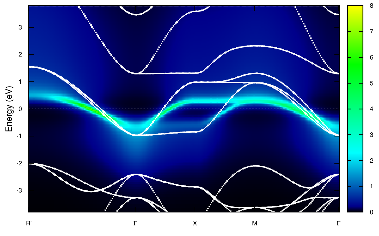
The white curve is the LDA band structure, the colored plot is the DMFT spectral function. One notes the renormalization of the bandwith as well as Hubbard bands, mainly visible a high energy (arount 2 eV). A more precise description of the Hubbard band would require a more converged calculation.

8 Electronic Structure of SrVO3: Conclusion

To sum up, the important physical parameters for DFT+DMFT are the definition of correlated orbitals, the choice of U and J (and double counting). The important technical parameters are the frequency and time grids as well as the number of steps for Monte Carlo, the DMFT loop and the DFT loop.

We showed in this tutorial how to compute the correlated orbital spectral functions, quasiparticle renormalization weights, total internal energy and the k-resolved spectral function.