Second tutorial on GW
Treatment of metals.
This tutorial aims at showing how to obtain self-energy corrections to the DFT Kohn-Sham eigenvalues within the GW approximation, in the metallic case, without the use of a plasmon-pole model. The band width and Fermi energy of Aluminum will be computed.
The user may read the papers
-
F. Bruneval, N. Vast, and L. Reining, Phys. Rev. B 74 , 045102 (2006) [Bruneval2006], for some information and results about the GW treatment of Aluminum. He will also find there an analysis of the effect of self-consistency on quasiparticles in solids (not present in this tutorial, however available in Abinit). The description of the contour deformation technique that bypasses the use of a plasmon-pole model to calculate the frequency convolution of G and W can be found in
-
S. Lebegue, S. Arnaud, M. Alouani, P. Bloechl, Phys. Rev. B 67, 155208 (2003) [Lebegue2003],
with the relevant formulas.
A brief description of the equations implemented in the code can be found in the GW notes Also, it is suggested to acknowledge the efforts of developers of the GW part of ABINIT, by citing the 2005 ABINIT publication.
The user should be familiarized with the four basic tutorials of ABINIT, see the tutorial index as well as the first GW tutorial.
Visualisation tools are NOT covered in this tutorial. Powerful visualisation procedures have been developed in the Abipy context, relying on matplotlib. See the README file of Abipy and the Abipy tutorials.
This tutorial should take about one hour to be completed (also including the reading of [Bruneval2006] and [Lebegue2003].
Note
Supposing you made your own installation of ABINIT, the input files to run the examples are in the ~abinit/tests/ directory where ~abinit is the absolute path of the abinit top-level directory. If you have NOT made your own install, ask your system administrator where to find the package, especially the executable and test files.
In case you work on your own PC or workstation, to make things easier, we suggest you define some handy environment variables by executing the following lines in the terminal:
export ABI_HOME=Replace_with_absolute_path_to_abinit_top_level_dir # Change this line
export PATH=$ABI_HOME/src/98_main/:$PATH      # Do not change this line: path to executable
export ABI_TESTS=$ABI_HOME/tests/             # Do not change this line: path to tests dir
export ABI_PSPDIR=$ABI_TESTS/Pspdir/  # Do not change this line: path to pseudos dir
Examples in this tutorial use these shell variables: copy and paste
the code snippets into the terminal (remember to set ABI_HOME first!) or, alternatively,
source the set_abienv.sh script located in the ~abinit directory:
source ~abinit/set_abienv.sh
The ‘export PATH’ line adds the directory containing the executables to your PATH so that you can invoke the code by simply typing abinit in the terminal instead of providing the absolute path.
To execute the tutorials, create a working directory (Work*) and
copy there the input files of the lesson.
Most of the tutorials do not rely on parallelism (except specific tutorials on parallelism). However you can run most of the tutorial examples in parallel with MPI, see the topic on parallelism.
The preliminary Kohn-Sham band structure calculation
Before beginning, you might consider to work in a different subdirectory as for the other tutorials. Why not Work_gw2?
In basic tutorial 4, we have computed different properties of Aluminum within DFT(LDA). Unlike for silicon, in this approximation, there is no outstanding problem in the computed band structure. Nevertheless, as you will see, the agreement of the band structure with experiment can be improved significantly if one uses the GW approximation.
In the directory Work_gw2, copy the file tgw2_1.abi located in $ABI_TESTS/tutorial/Input.
    mkdir Work_gw2
    cd Work_gw2
    cp $ABI_TESTS/tutorial/Input/tgw2_1.abi .
Then issue:
abinit tgw2_1.abi > tgw2_1.log 2> err &
# Crystalline aluminum
# Create the WFK file for the GW calculation.
ndtset    2

nband1    6
toldfe1   1.0d-8

iscf2       -2
getden2      1
nband2      35
nbdbuf2      5
tolwfr2     1.0d-10

#Definition of occupation numbers
occopt 3
tsmear 0.05

#Definition of the unit cell
acell 3*7.652

rprim  0.0  0.5  0.5   # FCC primitive vectors (to be scaled by acell)
       0.5  0.0  0.5
       0.5  0.5  0.0

#Definition of the atom types
ntypat 1
znucl 13

#Definition of the atoms
natom 1
typat 1
xred  0.0  0.0  0.0

#Definition of the planewave basis set
ecut  8.0

#Definition of the k-point grid
ngkpt       4 4 4

#64 k points
 nshiftk     1
 shiftk      0.  0.  0.
 istwfk     *1
#256 k points
#nshiftk 4
#shiftk 0 0 0   1/2 1/2 0   1/2 0 1/2  0 1/2 1/2
#istwfk     19*1

#Definition of the SCF procedure
nstep 50

prtvol     5
enunit     1


 pp_dirpath "$ABI_PSPDIR"
 pseudos "Psdj_nc_sr_04_pbe_std_psp8/Al.psp8"

##############################################################
# This section is used only for regression testing of ABINIT #
##############################################################
#%%<BEGIN TEST_INFO>
#%% [setup]
#%% executable = abinit
#%% test_chain = tgw2_1.abi, tgw2_2.abi, tgw2_3.abi, tgw2_4.abi
#%% [files]
#%% files_to_test =
#%%   tgw2_1.abo, tolnlines = 0, tolabs = 0.0e+00, tolrel = 0.0e+00
#%% [shell]
#%% post_commands =
#%%   ww_cp tgw2_1o_DS2_WFK tgw2_2i_WFK;
#%%   ww_cp tgw2_1o_DS2_WFK tgw2_3i_WFK;
#%%   ww_cp tgw2_1o_DS2_WFK tgw2_4i_WFK;
#%% [paral_info]
#%% max_nprocs = 4
#%% [extra_info]
#%% authors = F. Bruneval
#%% keywords = GW
#%% description =
#%%   Crystalline aluminum
#%%   Create the WFK file for the GW calculation.
#%%<END TEST_INFO>
This run generates the WFK file for the subsequent GW computation and also provides the band width of Aluminum. Note that the simple Fermi-Dirac smearing functional is used (occopt = 3), with a large smearing (tsmear = 0.05 Ha). The k-point grid is quite rough, an unshifted 4x4x4 Monkhorst-Pack grid (64 k-points in the full Brillouin Zone, folding to 8 k-points in the Irreducible wedge, ngkpt = 4 4 4). Converged results would need a 4x4x4 grid with 4 shifts (256 k-points in the full Brillouin zone). This grid contains the \(\Gamma\) point, at which the valence band structure reaches its minimum.
The output file presents the Fermi energy
Fermi (or HOMO) energy (eV) = 6.76526 Average Vxc (eV)= -9.88844
as well as the lowest energy, at the \(\Gamma\) point
 Eigenvalues (   eV  ) for nkpt=   8  k points:
 kpt#   1, nband=  6, wtk=  0.01563, kpt=  0.0000  0.0000  0.0000 (reduced coord)
  -4.22031   19.66151   19.66151   19.66151   21.09462   21.09462
So, the occupied band width is 10.98 eV within PBE. This is to be compared to the experimental value of 10.6 eV (see references in [Bruneval2006]).
Calculation of the screening file
Let’s run the calculation of the screening file immediately. So, copy the file tgw2_2.abi. Also, copy the WFK file (tgw2_1o_WFK) to tgw2_2i_WFK. Then run the calculation (it should take about 3 seconds).
    cp $ABI_TESTS/tutorial/Input/tgw2_2.abi .
    cp tgw2_1o_WFK tgw2_2i_WFK
    abinit tgw2_2.abi >& log &
# Crystalline aluminum :
# create the screening file

#Parameter for the screening calculation
optdriver    3
gwcalctyp    2
nband       30
ecuteps     4.0

nfreqim      4
nfreqre     10
freqremax    1.

#Definition of occupation numbers
occopt 3
tsmear 0.05

#Definition of the unit cell
acell 3*7.652

rprim  0.0  0.5  0.5   # FCC primitive vectors (to be scaled by acell)
       0.5  0.0  0.5
       0.5  0.5  0.0

#Definition of the atom types
ntypat 1
znucl 13

#Definition of the atoms
natom 1
typat 1
xred  0.0  0.0  0.0

#Definition of the planewave basis set
ecut  8.0

#Definition of the k-point grid
ngkpt        4 4 4
nshiftk      1
shiftk       0.  0.  0.
istwfk       *1

#Definition of the SCF procedure
nstep       50
toldfe      1.0d-8

prtvol     5
enunit     1


 pp_dirpath "$ABI_PSPDIR"
 pseudos "Psdj_nc_sr_04_pbe_std_psp8/Al.psp8"

##############################################################
# This section is used only for regression testing of ABINIT #
##############################################################
#%%<BEGIN TEST_INFO>
#%% [setup]
#%% executable = abinit
#%% test_chain = tgw2_1.abi, tgw2_2.abi, tgw2_3.abi, tgw2_4.abi
#%% [files]
#%% files_to_test =
#%%   tgw2_2.abo, tolnlines= 32, tolabs=  1.1e-02, tolrel=  2.0e-00
#%% [shell]
#%% post_commands =
#%%   ww_cp tgw2_2o_SCR tgw2_3i_SCR;
#%%   ww_cp tgw2_2o_SCR tgw2_4i_SCR
#%% [paral_info]
#%% max_nprocs = 4
#%% [extra_info]
#%% authors = F. Bruneval
#%% keywords = GW
#%% description =
#%%   Crystalline aluminum:
#%%   create the screening file
#%%<END TEST_INFO>
We now have to consider starting a GW calculation. However, unlike in the case of Silicon in the previous GW tutorial, where we were focussing on quantities close to the Fermi energy (spanning a range of a few eV), here we need to consider a much wider range of energy: the bottom of the valence band lies around -11 eV below the Fermi level. Unfortunately, this energy is of the same order of magnitude as the plasmon excitations. With a rough evaluation, the classical plasma frequency for a homogeneous electron gas with a density equal to the average valence density of Aluminum is 15.77 eV. Hence, using plasmon-pole models may be not really appropriate.
In what follows, we will compute the GW band structure without a plasmon-pole model, by performing the numerical frequency convolution. In practice, it is convenient to extend all the functions of frequency to the full complex plane. And then, making use of the residue theorem, the integration path can be deformed: one transforms an integral along the real axis into an integral along the imaginary axis plus residues enclosed in the new contour of integration. The method is extensively described in [Lebegue2003].
Examine the input file tgw2_2.abi.
# Crystalline aluminum :
# create the screening file

#Parameter for the screening calculation
optdriver    3
gwcalctyp    2
nband       30
ecuteps     4.0

nfreqim      4
nfreqre     10
freqremax    1.

#Definition of occupation numbers
occopt 3
tsmear 0.05

#Definition of the unit cell
acell 3*7.652

rprim  0.0  0.5  0.5   # FCC primitive vectors (to be scaled by acell)
       0.5  0.0  0.5
       0.5  0.5  0.0

#Definition of the atom types
ntypat 1
znucl 13

#Definition of the atoms
natom 1
typat 1
xred  0.0  0.0  0.0

#Definition of the planewave basis set
ecut  8.0

#Definition of the k-point grid
ngkpt        4 4 4
nshiftk      1
shiftk       0.  0.  0.
istwfk       *1

#Definition of the SCF procedure
nstep       50
toldfe      1.0d-8

prtvol     5
enunit     1


 pp_dirpath "$ABI_PSPDIR"
 pseudos "Psdj_nc_sr_04_pbe_std_psp8/Al.psp8"

##############################################################
# This section is used only for regression testing of ABINIT #
##############################################################
#%%<BEGIN TEST_INFO>
#%% [setup]
#%% executable = abinit
#%% test_chain = tgw2_1.abi, tgw2_2.abi, tgw2_3.abi, tgw2_4.abi
#%% [files]
#%% files_to_test =
#%%   tgw2_2.abo, tolnlines= 32, tolabs=  1.1e-02, tolrel=  2.0e-00
#%% [shell]
#%% post_commands =
#%%   ww_cp tgw2_2o_SCR tgw2_3i_SCR;
#%%   ww_cp tgw2_2o_SCR tgw2_4i_SCR
#%% [paral_info]
#%% max_nprocs = 4
#%% [extra_info]
#%% authors = F. Bruneval
#%% keywords = GW
#%% description =
#%%   Crystalline aluminum:
#%%   create the screening file
#%%<END TEST_INFO>
The ten first lines contain the important information. There, you find some input variables that you are already familiarized with, like optdriver, ecuteps, but also new input variables: gwcalctyp, nfreqim, nfreqre, and freqremax. The purpose of this run is simply to generate the screening matrices. Unlike for the plasmon-pole models, one needs to compute these at many different frequencies. This is the purpose of the new input variables. The main variable gwcalctyp is set to 2 in order to specify a non plasmon-pole model calculation. Note that the number of frequencies along the imaginary axis governed by nfreqim can be chosen quite small, since all functions are smooth in this direction. In contrast, the number of frequencies needed along the real axis set with the variable nfreqre is usually larger.
Finding the Fermi energy and the bottom of the valence band
Let’s run the calculation of the band width immediately and then we’ll study of the input file. So, get the file tgw2_3.abi.
    cp $ABI_TESTS/tutorial/Input/tgw2_3.abi .
    cp tgw2_1o_WFK tgw2_3i_WFK
    cp tgw2_2o_SCR tgw2_3i_SCR
    abinit tgw2_3.abi >& log &
The computation of the GW quasiparticle energy at the \(\Gamma\) point of Aluminum does not differ from the one of quasiparticle in Silicon. However, the determination of the Fermi energy raises a completely new problem: one should sample the whole Brillouin Zone to get new energies (quasiparticle energies) and then determine the Fermi energy. This is actually the first step towards a self-consistency!
Examine the input file tgw2_3.abi:
# Crystalline aluminum :
# calculation of the quasi-particle Fermi energy

#Parameters for the GW calculation
optdriver    4
nband       30
ecutsigx    8.0

gwcalctyp   12
symsigma     0

nkptgw       8
kptgw
      0.000000    0.000000    0.000000
      0.250000    0.000000    0.000000
      0.500000    0.000000    0.000000
      0.250000    0.250000    0.000000
      0.500000    0.250000    0.000000
     -0.250000    0.250000    0.000000
      0.500000    0.500000    0.000000
     -0.250000    0.500000    0.250000
bdgw
             1 1
             2 2
             1 2
             1 1
             1 3
             1 3
             1 5
             1 4


#Definition of occupation numbers
occopt 3
tsmear 0.05

#Definition of the unit cell
acell 3*7.652

rprim  0.0  0.5  0.5   # FCC primitive vectors (to be scaled by acell)
       0.5  0.0  0.5
       0.5  0.5  0.0

#Definition of the atom types
ntypat 1
znucl 13

#Definition of the atoms
natom 1
typat 1
xred  0.0  0.0  0.0

#Definition of the planewave basis set
ecut  8.0

#Definition of the k-point grid
ngkpt         4 4 4
nshiftk       1
shiftk        0.  0.  0.
istwfk        *1

#Definition of the SCF procedure
nstep 50
toldfe 1.0d-8

prtvol     5
enunit     1

 pp_dirpath "$ABI_PSPDIR"
 pseudos "Psdj_nc_sr_04_pbe_std_psp8/Al.psp8"

##############################################################
# This section is used only for regression testing of ABINIT #
##############################################################
#%%<BEGIN TEST_INFO>
#%% [setup]
#%% executable = abinit
#%% test_chain = tgw2_1.abi, tgw2_2.abi, tgw2_3.abi, tgw2_4.abi
#%% [files]
#%% files_to_test =
#%%   tgw2_3.abo, tolnlines=  5, tolabs=0.002, tolrel=  3.000e-02
#%% [paral_info]
#%% max_nprocs = 4
#%% [extra_info]
#%% authors = F. Bruneval
#%% keywords = GW
#%% description =
#%%   Crystalline aluminum:
#%%   calculation of the quasi-particle Fermi energy
#%%<END TEST_INFO>
The first thirty lines contain the important information. There, you find some input variables with values that you are already familiarized with, like optdriver, ecutsigx, ecutwfn. Then, comes the input variable gwcalctyp = 12. The value x2 corresponds to a contour integration. The value 1x corresponds to a self-consistent calculation with update of the energies only. Then, one finds the list of k points and bands for which a quasiparticle correction will be computed: nkptgw, kptgw, and bdgw. The number and list of k-points is simply the same as nkpt and kpt. One might have specified less k-points, though (only those needing an update). The list of band ranges bdgw has been generated on the basis of the DFT(LDA) eigenenergies. We considered only the bands in the vicinity of the Fermi level: bands much below or much above are likely to remain much below or much above the Fermi region. In the present run, we are just interested in the states that may cross the Fermi level, when going from DFT to GW. Of course, it would have been easier to select an homogeneous range for the whole Brillouin zone, e.g. from 1 to 5, but this would have been more time-consuming.
In the output file, one finds the quasiparticle energy at \(\Gamma\), for the lowest band:
--- !SelfEnergy_ee
iteration_state: {dtset: 1, }
kpoint     : [   0.000,    0.000,    0.000, ]
spin       : 1
KS_gap     :    0.000
QP_gap     :    0.000
Delta_QP_KS:    0.000
data: !SigmaeeData |
     Band     E_DFT   <VxcDFT>   E(N-1)  <Hhartree>   SigX  SigC[E(N-1)]    Z     dSigC/dE  Sig[E(N)]  DeltaE  E(N)_pert E(N)_diago
        1    -4.220    -9.458    -4.220     5.238   -15.616     5.931     0.903    -0.107    -9.663    -0.206    -4.426    -4.448
        2    19.662    -9.585    19.662    29.246    -2.718    -7.097     0.802    -0.246    -9.770    -0.185    19.477    19.430
        3    19.662    -9.585    19.662    29.246    -2.718    -7.098     0.802    -0.247    -9.770    -0.185    19.476    19.430
        4    19.662    -9.585    19.662    29.246    -2.718    -7.098     0.802    -0.247    -9.770    -0.185    19.476    19.431
        5    21.095    -9.387    21.095    30.482    -2.461    -7.390     0.713    -0.402    -9.718    -0.331    20.764    20.631
        6    21.095    -9.387    21.095    30.482    -2.461    -7.390     0.713    -0.402    -9.718    -0.331    20.764    20.631
        7    21.095    -9.387    21.095    30.482    -2.461    -7.390     0.713    -0.403    -9.718    -0.331    20.764    20.631
...
(the last column is the relevant quantity). The updated Fermi energy is also mentioned:
New Fermi energy : 2.425933E-01 Ha , 6.601299E+00 eV
The last information is not printed in case of gwcalctyp lower than 10.
Combining the quasiparticle energy at \(\Gamma\) and the Fermi energy, gives the band width, 11.05 eV. Remember the experimental value is around 10.6 eV.
Computing a GW spectral function, and the plasmon satellite of Aluminum
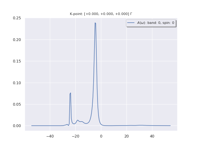
The access to the non-plasmon-pole-model self-energy (real and imaginary part) has additional benefit, e.g. an accurate spectral function can be computed, see [Lebegue2003]. You may be interested to see the plasmon satellite of Aluminum, which can be accounted for within the GW approximation.
Remember that the spectral function is proportional to (with some multiplicative matrix elements) the spectrum which is measured in photoemission spectroscopy (PES). In PES, a photon impinges the sample and extracts an electron from the material. The difference of energy between the incoming photon and the obtained electron gives the binding energy of the electron in the solid, or in other words the quasiparticle energy or the band structure. In simple metals, an additional process can take place easily: the impinging photon can extract an electron together with a global charge oscillation in the sample. The extracted electron will have a kinetic energy lower than in the direct process, because a part of the energy has gone to the plasmon. The electron will appear to have a larger binding energy… You will see that the spectral function of Aluminum consists of a main peak which corresponds to the quasiparticle excitation and some additional peaks which correspond to quasiparticle and plasmon excitations together.
Let’s run this calculation immediately:
    cp $ABI_TESTS/tutorial/Input/tgw2_4.abi .
    cp tgw2_1o_WFK tgw2_4i_WFK
    cp tgw2_2o_SCR tgw2_4i_SCR
    abinit tgw2_4.abi >& log &
# Crystalline aluminum : perform the GW calculation
# at the bottom of the valence band
# Obtain the corresponding spectral function

#Parameters for the GW calculation

optdriver    4
gwcalctyp    2
symsigma     0
nband       30
ecutsigx    8.0

nfreqsp    200
freqspmax    2.

nkptgw       1
kptgw
             0.000000    0.000000    0.000000
bdgw
             1 1

#Definition of occupation numbers
occopt 3
tsmear 0.05

#Definition of the unit cell
acell 3*7.652

rprim  0.0  0.5  0.5   # FCC primitive vectors (to be scaled by acell)
       0.5  0.0  0.5
       0.5  0.5  0.0

#Definition of the atom types
ntypat 1
znucl 13

#Definition of the atoms
natom 1
typat 1
xred  0.0  0.0  0.0

#Definition of the planewave basis set
ecut  8.0

#Definition of the k-point grid
ngkpt         4 4 4
nshiftk       1
shiftk        0.  0.  0.
istwfk        *1


prtvol     5
enunit     1


 pp_dirpath "$ABI_PSPDIR"
 pseudos "Psdj_nc_sr_04_pbe_std_psp8/Al.psp8"

##############################################################
# This section is used only for regression testing of ABINIT #
##############################################################
#%%<BEGIN TEST_INFO>
#%% [setup]
#%% executable = abinit
#%% test_chain = tgw2_1.abi, tgw2_2.abi, tgw2_3.abi, tgw2_4.abi
#%% [files]
#%% files_to_test =
#%%   tgw2_4.abo, tolnlines=  2, tolabs=  1.1e-03, tolrel=  3.0e-02
#%% [paral_info]
#%% max_nprocs = 4
#%% [extra_info]
#%% authors = F. Bruneval
#%% keywords = GW
#%% description =
#%%   Crystalline aluminum : perform the GW calculation
#%%   at the bottom of the valence band
#%%   Obtain the corresponding spectral function
#%%<END TEST_INFO>
Compared to the previous file (tgw2_3.abi), the input file contains two additional keywords: nfreqsp, and freqspmax. Also, the computation of the GW self-energy is done only at the \(\Gamma\) point.
The spectral function is written in the file tgw2_4o_SIG. It is a simple text file. It contains, as a function of the frequency (eV), the real part of the self-energy, the imaginary part of the self-energy, and the spectral function. You can visualize it using your preferred software. For instance, start gnuplot and issue
p 'tgw2_4o_SIG' u 1:4 w l
You should be able to distinguish the main quasiparticle peak located at the GW energy (-3.7 eV) and some additional features in the vicinity of the GW eigenvalue minus a plasmon energy (-3.7 eV - 15.8 eV = -19.5 eV).
Tip
If AbiPy is installed on your machine, you can use the abiopen.py script
with the --expose option to visualize the results:
abiopen.py tgw2_4o_SIGRES.nc -e -sns
Another file, tgw2_4o_GW, is worth to mention: it contains information to be used for the subsequent calculation of excitonic effects within the Bethe-Salpeter Equation with ABINIT or with other codes from the ETSF software page.