Parallelism for molecular dynamics

How to perform Molecular Dynamics calculations using parallelism

This tutorial aims at showing how to perform molecular dynamics with ABINIT using a parallel computer. You will learn how to launch molecular dynamics calculation and what are the main input variables that govern convergence and numerical efficiency.

You are supposed to know already some basics of parallelism in ABINIT, explained in the tutorial A first introduction to ABINIT in parallel, and parallelism over bands and plane waves.

This tutorial should take about 1.5 hour to be done and requires to have at least a 200 CPU core parallel computer.

Note

Supposing you made your own installation of ABINIT, the input files to run the examples are in the ~abinit/tests/ directory where ~abinit is the absolute path of the abinit top-level directory. If you have NOT made your own install, ask your system administrator where to find the package, especially the executable and test files.

In case you work on your own PC or workstation, to make things easier, we suggest you define some handy environment variables by executing the following lines in the terminal:

export ABI_HOME=Replace_with_absolute_path_to_abinit_top_level_dir # Change this line
export PATH=$ABI_HOME/src/98_main/:$PATH      # Do not change this line: path to executable
export ABI_TESTS=$ABI_HOME/tests/             # Do not change this line: path to tests dir
export ABI_PSPDIR=$ABI_TESTS/Pspdir/  # Do not change this line: path to pseudos dir

Examples in this tutorial use these shell variables: copy and paste the code snippets into the terminal (remember to set ABI_HOME first!) or, alternatively, source the set_abienv.sh script located in the ~abinit directory:

source ~abinit/set_abienv.sh

The ‘export PATH’ line adds the directory containing the executables to your PATH so that you can invoke the code by simply typing abinit in the terminal instead of providing the absolute path.

To execute the tutorials, create a working directory (Work*) and copy there the input files of the lesson.

Most of the tutorials do not rely on parallelism (except specific tutorials on parallelism). However you can run most of the tutorial examples in parallel with MPI, see the topic on parallelism.

Tip

In this tutorial, most of the images and plots are easily obtained using the post-processing tool qAgate or agate, its core engine. Any post-process tool will work though !!

Summary of the molecular dynamics method

The basic idea underlying Ab Initio Molecular Dynamics (AIMD) is to compute the forces acting on the nuclei from electronic structure calculations that are performed as the molecular dynamics trajectory is generated.

An AIMD calculation assumes only that the system is composed of nuclei and electrons, that the Born -Oppenheimer approximation is valid, and that the dynamics of the nuclei can be treated classically on the ground-state electronic surface. It allows both equilibrium thermodynamic and dynamical properties of a system at finite temperature to be computed. For example melting temperatures, phase transitions, atomic vibrations, structure factor… but also XANES or IR spectrum can be obtained with this technique.

AIMD deals with supercells of hundred to thousand of atoms (usually, the larger, the better!). In addition Molecular Dynamics simulations can be performed for days, weeks or even months! They are therefore very time consuming and can not be done without the help of high speed and massively parallel computing.

In the following, when “run ABINIT over nn CPU cores” appears, you have to use a specific command line according to the operating system and architecture of the computer you are using. This can be for instance: mpirun -n nn abinit input.abi or the use of a specific submission file.

For this tutorial, one needs a working directory. Why not Work_paral_moldyn? e.g. with the commands:

mkdir -p $ABI_TESTS/tutoparal/Input/Work_paral_moldyn
cd $ABI_TESTS/tutoparal/Input/Work_paral_moldyn

Performing molecular dynamics with ABINIT

There are different algorithms to do molecular dynamics. See the input variable ionmov, with values 1, 6, 7, 8, 9, 12, 13 and 14. dtion controls the ion time step in atomic units of time (one atomic time unit is 2.418884 x 10^-17 seconds, which is the value of Planck’s constant in Ha.s). The default value is 100. You should try several values for dtion in order to establish the stable and efficient choice. For example this value should decrease at high pressure.

Except for the isothermal/isenthalpic (ionmov 13) ensemble the input variable optcell must be 0 (default value). You have also to define the maximal number of timesteps of the molecular dynamics.

Usually you can set the input variable ntime to a large value, 5000, since there is no end to a molecular dynamics simulation. You can always stop or restart the calculation at your convenience by using the input variable restartxf=-1.

The input file tmoldyn_01.abi is an example of a file that contains data for a molecular dynamics simulation using the isokinetic ensemble ionmov=12 for fcc aluminum.

View tests/tutoparal/Input/tmoldyn_01.abi

Open the tmoldyn_01.abi file and look at it carefully. The unit cell is defined at the end. It is a 2x2x2 fcc supercell containing 32 atoms of Al. ionmov is set to 12 for the isokinetic ensemble, and since ntime is set to 50, ABINIT will carry on 50 time steps of molecular dynamics. The calculation will be performed for a temperature of 3000 K, see the key variable mdtemp. It gives the initial and final temperatures of the simulation (in Kelvin). The temperature will change linearly from the initial temperature mdtemp(1) at itime=1 to the final temperature mdtemp(2) at the end of the ntime timesteps. Here the temperature will stay constant during the whole simulation.

Note

Note that we use the same temperature for the ions and the electrons: occopt has been set to 3 for a Fermi-Dirac smearing and tsmear has been set to 3000 Kelvin. Nothing prevents you to use different electronic and ionic temperature, you just have to know why you are doing so! With such a temperature, the number of electronic bands nband is set to 80.

Note

For AIMD, nsym is set to 1 to remove the use of symmetries !

Molecular dynamics simulations are always large calculations, dealing with supercells of hundreds to thousands of atoms. Therefore they are always performed in parallel. In tmoldyn_01.in, paral_kgb has been set to 1 to activate the parallelisation over k-points, G-vectors and bands. The three following keywords give the number of processors for each level of parallelisation. Since we have only 1 k-point in the simulation (ngkpt has been set to 1 1 1) np_spkpt is set to 1, npband to 2 with bandpp=40 (1 unique block), and npfft is kept to 1.

Then run the calculation in parallel over 2 CPU cores. You can change the distribution of processors over the level of parallelisation to try to find the most efficient one. Since molecular dynamics can last for weeks, it is crucial to find the appropriate distribution to reduce the computational time at the maximum. You can use timopt to get information on time repartition during the simulation.

Now look at the output file. For each iteration you will see the coordinates, the forces, the velocities and the kinetic and the total energy.

In addition, ABINIT should have generated a _HIST.nc file, which contains the whole history of the molecular dynamics simulation: atomic positions, velocities, primitive translations, stress tensor, energies… at each time step. This file will be used to restart the calculation if you want to perform more time steps or to extract the necessary informations to make use of the molecular dynamics simulation. In tmoldyn_01.abi add the keyword restartxf and set it to -1. Run the calculation again, in the same directory. Look at the new output file. The number of each time step are indicated over the total number of steps:

Iteration: (  1/100) Internal Cycle: (1/1)

Since we already performed 50 steps of molecular dynamics, the total number of time steps are now 100. So the first 50 iterations are from the previous calculation. You can check that by comparing tmoldyn_01.abo and tmoldyn_01.abo0001. There is only one _HIST.nc file and it contains the history of the two calculations.

Now we can calculate and plot several quantities.

We need for that the diag_moldyn.py python script. You can find it in the $ABI_HOME/doc/tutorial/paral_moldyn_assets directory (link here). Run the script as:

python diag_moldyn.py

Warning

The above script diag_moldyn.py uses python2 and does not work with python3

You can read (on standard output) the average value and the standard deviation of the total energy, the temperature and the pressure. You have also generated several files which contain pressures, energies, stresses, positions and temperatures. You can plot this files to observe the behavior of the quantities during the molecular dynamics. Note that 100 time steps is far from being sufficient to equilibrate physical quantities as pressure. 2000 or 3000 are more common numbers to reach this goal but it would exceed the time allocated for this tutorial.

Tip

You can use agate or qAgate to open and visualize the _HIST.nc file. In the console, the averages and the standard deviations of several quantities like temperature pressure stresses are automatically displayed.

You can plot the evolution of pressure with respect to the time step by issuing :plot P. Replace :plot by :print or :data to save the image or write an ASCII file.

The convergence on k-points and supercell size

In the previous section you have learned to perform molecular dynamics with abinit. We used a fcc supercell of 32 atoms with only 1 k-point. In this section we will make convergence studies with respect to these parameters.

Computing the convergence in k-points

The files tmoldyn_02.abi and tmoldyn_03.abi are input files for 2x2x2 and 3x3x3 k-points grid respectively (4 and 14 k-points in the irreducible Brillouin zone).

View tests/tutoparal/Input/tmoldyn_02.abi View tests/tutoparal/Input/tmoldyn_03.abi

Since the parallelisation is the most efficient over the k-point level you should always put nkpt to the largest possible value before increasing npfft and npband. We have followed this rule in the input files.

If you used the diag_moldyn.py script, change the name of the previous file PRESS to PRESS01 to save it. Run now ABINIT in parallel over 8 CPU cores with tmoldyn_02.abi and over 28 CPU cores with tmoldyn_03.abi. At the end of each calculation use the diag_moldyn.py script and save the results in PRESS02 and PRESS03. You can now plot the pressures in term of the k-points grids and compare the average values:

Tip

Alternatively, use agate or qagate to directly produce the following picture

:open tmoldyn_01o_HIST.nc
:plot P hold=true
:open tmoldyn_02o_HIST.nc
:plot P 
:open tmoldyn_03o_HIST.nc
:plot P  output Kpoints

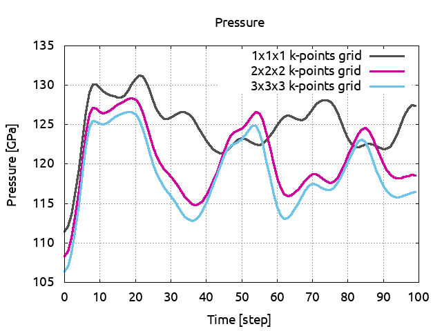
As said previously our simulations are too short to be completely convincing but you can see that you need at least a 2x2x2 k-points grid for a 32 atoms cell. If you have some time, increase ntime to 300 and run again ABINIT.

Computing the convergence in cell size

We also have to check if our cell is sufficiently large to give reliable physical quantities. In the previous section we used a 2x2x2 fcc supercell. tmoldyn_04.abi is an input file for a 3x3x3 fcc supercell and therefore contains 108 atoms. nband and acell has been scaled accordingly to take into account the new size of the cell.

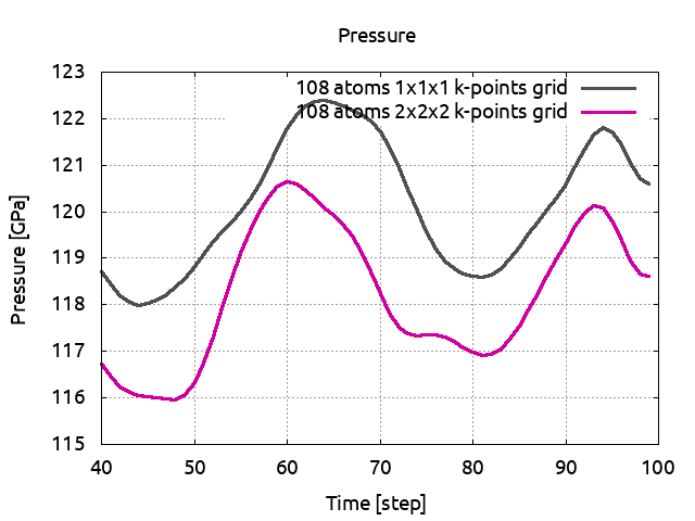
Run now ABINIT in parallel over 8 CPU cores and then diag_moldyn.py (note that the output file is very big, and no reference has been provided for comparison). Save the pressure to PRESS04. tmoldyn_05.abi has the same cell but a 2x2x2 k-points grid (note that the output file is very big, and no reference has been provided for comparison). Run it over the adequate number of cores and save the pressure to PRESS05. Plot now PRESS04 and PRESS05 and compare the average values. You will see that for this size of cell, one k-point is sufficient.

Tip

Alternatively, use agate or qagate to directly produce the following picture

:open tmoldyn_04o_HIST.nc
:plot P  hold=true
:open tmoldyn_05o_HIST.nc
:plot P

We are now going to increase again the cell size. With a 4x4x4 fcc cell, the file tmoldyn_06.in has 256 atoms. Of course, nband and acell have been scaled. This calculation should last for 50 min over 32 CPU cores (note that the output file is very big, and no reference has been provided for comparison). Run it and save the pressure to PRESS06. Plot now PRESS02, PRESS04 and PRESS06, remove the first steps and compare the pressure average values:

Tip

Alternatively, use agate or qagate to directly produce the following picture

:open tmoldyn_02o_HIST.nc
:plot P  hold=true
:open tmoldyn_05o_HIST.nc
:plot P
:open tmoldyn_06o_HIST.nc
:plot P  

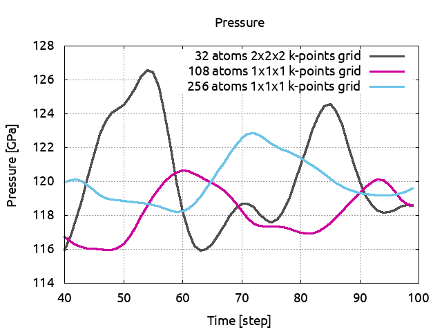
You can see that even if the pressure was converged in term of k-points, the 32 atoms supercell was not sufficient to give a reliable pressure. A 3x3x3 supercell with only 1 k-point seems to be the adequate size. You see also that with a bigger cell, the pressure fluctuations are considerably reduced.

Note that here we made the convergence studies using the pressure as a criteria. The results can depend on the physical quantity you are looking at, pressure, temperature, energy, or dynamical matrices by observing the displacement fluctuations.... Always check if your cell is large enough and give the corresponding uncertainty. Also, to reduce the time necessary to do this tutorial we set the value of ecut to 3 Ha. This is too small, for Al, it should be closer to 8 Ha.

Finally, here and for simplicity, we just changed the value of ngkpt to change the grid of k-points. By default, ABINIT uses a shiftk so the one k-point generated with a 1x1x1 gid is not \(\Gamma\)!. To get the \(\Gamma\) point only, and decrease the execution time by half, set shiftk to 0 0 0 and check the value kpt in the output file.

Compute the melting temperature of Al at a given pressure

As an example of what can be done in molecular dynamics, we are going to calculate the melting temperature of aluminum using the so-called Heat Until it Melts (HUM) method. In this method the solid phase is heated gradually until melting occurs. Let’s start with a temperature of 4500 K. To work fast, we use a 32 atoms supercell and 1 k-point (note that the output file is very big, and no reference has been provided for comparison).

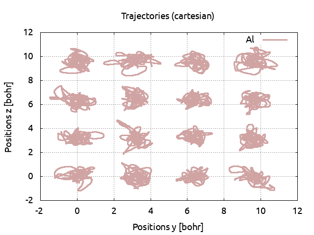
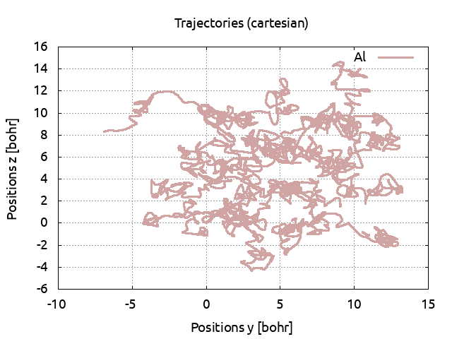
Run ABINIT in parallel over 2 CPU cores and then diag_moldyn.py. Save the pressure to PRESS71. Plot the atomic positions, you see that at this temperature, the cell is solid.

Tip

Alternatively, use agate or qagate to directly produce the following pictures. The positions can be obtains directly with :plot positions yz where yz can be replaced by xy or xz to change the plan. Note that the atoms on the border are not displayed at contrario to the animations.

Increase the temperature to 5000 K (do not forget to also change the electronic temperature with tsmear) and run ABINIT. Save the pressure and again, look at the positions. The cell is still solid. Set the temperature to 5500 K. Look at the positions: the ions are moving across the cell and do not come back to their equilibrium positions. The cell has melted and is now liquid. Plot the pressures for the three simulations:

Tip

To run the three temperatures in 1 run, use ndtset 3 and specify for each dtset the values for mdtemp and tsmear. An example of file is given with tmoldyn_07.abi.

View tests/tutoparal/Input/tmoldyn_07.abi

Tip

To produce the following plot, use agate or qagate with the following commands

:open tmoldyn_07o_DS1_HIST.nc
:plot P hold=true
:open tmoldyn_07o_DS2_HIST.nc
:plot P 
:open tmoldyn_07o_DS3_HIST.nc
:plot P 

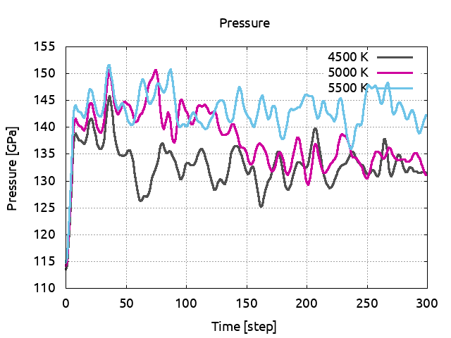
You can clearly observe a discontinuous change in pressure due to the volume difference between the solid and liquid phases. This give a melting temperature of 5250 K at 132 GPa. One has to be very careful. Indeed, in addition to the crude parameters we used (ecut, natom…), the HUM method has some intrinsic drawbacks. In HUM the crystal is heated homogeneously, the melting initiates in the bulk and this results in an overheating effect.