Third tutorial
Crystalline silicon.
This tutorial aims at showing you how to get the following physical properties, for an insulator:
- the total energy,
- the lattice parameter,
- the band structure (actually, the Kohn-Sham band structure).
You will learn about the use of k-points, as well as the smearing of the plane-wave kinetic energy cut-off.
You will also use the powerful visualisation procedures that have been developed in the Abipy context, relying on matplotlib. See the README of Abipy and the Abipy tutorials. Other visualization tools are available, but will not be covered.
This tutorial should take about 1 hour.
Note
Supposing you made your own installation of ABINIT, the input files to run the examples are in the ~abinit/tests/ directory where ~abinit is the absolute path of the abinit top-level directory. If you have NOT made your own install, ask your system administrator where to find the package, especially the executable and test files.
In case you work on your own PC or workstation, to make things easier, we suggest you define some handy environment variables by executing the following lines in the terminal:
export ABI_HOME=Replace_with_absolute_path_to_abinit_top_level_dir # Change this line
export PATH=$ABI_HOME/src/98_main/:$PATH      # Do not change this line: path to executable
export ABI_TESTS=$ABI_HOME/tests/             # Do not change this line: path to tests dir
export ABI_PSPDIR=$ABI_TESTS/Pspdir/  # Do not change this line: path to pseudos dir
Examples in this tutorial use these shell variables: copy and paste
the code snippets into the terminal (remember to set ABI_HOME first!) or, alternatively,
source the set_abienv.sh script located in the ~abinit directory:
source ~abinit/set_abienv.sh
The ‘export PATH’ line adds the directory containing the executables to your PATH so that you can invoke the code by simply typing abinit in the terminal instead of providing the absolute path.
To execute the tutorials, create a working directory (Work*) and
copy there the input files of the lesson.
Most of the tutorials do not rely on parallelism (except specific tutorials on parallelism). However you can run most of the tutorial examples in parallel with MPI, see the topic on parallelism.
Computing the total energy of silicon at a fixed number of k-points
Before beginning, you might consider working in a different subdirectory, as for tutorial 1 or 2. Why not Work3?
The following commands will move you to your working directory, create the Work3 directory, and move you into that directory as you did in the first and second tutorials. Then, we copy the file tbase3_1.abi inside the Work3 directory. The commands are:
cd $ABI_TESTS/tutorial/Input
mkdir Work3
cd Work3
cp ../tbase3_1.abi .
This is your input file:
# Crystalline silicon : computation of the total energy
#

#Definition of the unit cell
acell 3*10.18          # This is equivalent to   10.18 10.18 10.18
rprim  0.0  0.5  0.5   # In tutorials 1 and 2, these primitive vectors
       0.5  0.0  0.5   # (to be scaled by acell) were 1 0 0  0 1 0  0 0 1
       0.5  0.5  0.0   # that is, the default.

#Definition of the atom types
ntypat 1          # There is only one type of atom
znucl 14          # The keyword "znucl" refers to the atomic number of the
                  # possible type(s) of atom. The pseudopotential(s)
                  # mentioned in the "files" file must correspond
                  # to the type(s) of atom. Here, the only type is Silicon.
pp_dirpath "$ABI_PSPDIR"        # This is the path to the directory were
                                # pseudopotentials for tests are stored
pseudos "Psdj_nc_sr_04_pw_std_psp8/Si.psp8"
                                # Name and location of the pseudopotential

#Definition of the atoms
natom 2           # There are two atoms
typat 1 1         # They both are of type 1, that is, Silicon.
xred              # This keyword indicate that the location of the atoms
                  # will follow, one triplet of number for each atom
   0.0  0.0  0.0  # Triplet giving the REDUCED coordinate of atom 1.
   1/4  1/4  1/4  # Triplet giving the REDUCED coordinate of atom 2.
                  # Note the use of fractions (remember the limited
                  # interpreter capabilities of ABINIT)

#Definition of the planewave basis set
ecut  12.0         # Maximal kinetic energy cut-off, in Hartree

#Definition of the k-point grid
kptopt 1          # Option for the automatic generation of k points, taking
                  # into account the symmetry
ngkpt 2 2 2       # This is a 2x2x2 grid based on the primitive vectors
nshiftk 4         # of the reciprocal space (that form a BCC lattice !),
                  # repeated four times, with different shifts :
shiftk 0.5 0.5 0.5
       0.5 0.0 0.0
       0.0 0.5 0.0
       0.0 0.0 0.5
                  # In cartesian coordinates, this grid is simple cubic, and
                  # actually corresponds to the
                  # so-called 4x4x4 Monkhorst-Pack grid

#Definition of the SCF procedure
nstep 10          # Maximal number of SCF cycles
toldfe 1.0d-6     # Will stop when, twice in a row, the difference
                  # between two consecutive evaluations of total energy
                  # differ by less than toldfe (in Hartree)
                  # This value is WAY TOO LARGE for most realistic studies of materials
diemac 12.0       # Although this is not mandatory, it is worth to
                  # precondition the SCF cycle. The model dielectric
                  # function used as the standard preconditioner
                  # is described in the "dielng" input variable section.
                  # Here, we follow the prescription for bulk silicon.

##############################################################
# This section is used only for regression testing of ABINIT #
##############################################################
#%%<BEGIN TEST_INFO>
#%% [setup]
#%% executable = abinit
#%% [files]
#%% files_to_test =
#%%   tbase3_1.abo, tolnlines=  0, tolabs=  0.000e+00, tolrel=  0.000e+00
#%% [paral_info]
#%% max_nprocs = 4
#%% [extra_info]
#%% authors = Unknown
#%% keywords =
#%% description = Crystalline silicon: computation of the total energy
#%%<END TEST_INFO>
You should edit it, read it carefully, have a look at the following new input variables and their explanation:
- rprim
- xred (used instead of xcart)
- kptopt, ngkpt, nshiftk, shiftk, kptrlatt (not easy, take your time!)
- diemac (with respect to previous calculations where isolated molecules were considered, a different value is used for this variable).
Note also the following: you will work at fixed ecut (12Ha). It is implicit that in real life, you should do a convergence test with respect to ecut. Here, a suitable ecut is given to you; it corresponds to the suggested ecut for this pseudopotential according to the PseudoDojo website where the silicon pseudopotential was taken. When we will relax the lattice parameter, it will result in a lattice parameter that is 0.2% off of the experimental value. Such convergence study has to be made for each physical property that is the target of your interest. While the value of ecut giving converged properties usually do not depend much on the property, this is not true for the convergence with respect to k points.
When you have read the input file, you can run the code, as usual:
abinit tbase3_1.abi > log 2> err &
Then, read the output file, and note the total energy:
etotal -8.5187390642E+00
Starting the convergence study with respect to k-points
There is, of course, a convergence study associated with the sampling of the Brillouin zone. You should examine different grids, of increasing resolution. You might try the following series of grids:
ngkpt1  2 2 2
ngkpt2  4 4 4
ngkpt3  6 6 6
ngkpt4  8 8 8
However, the associated number of k-points in the irreducible Brillouin zone grows very fast. It is
nkpt1  2
nkpt2 10
nkpt3 28
nkpt4 60
Abinit computes automatically this number of k-points, from the definition of the grid and the symmetries. You might nevertheless define an input nkpt value in the input file, in which case the code will compare its computed value (from the grid) with this input value.
We take this opportunity to examine the behaviour of abinit when a problem is detected. Let us suppose that with ngkpt 4 4 4, one mentions nkpt 2. The input file tbase3_2.abi is an example:
# Crystalline silicon : computation of the total energy
#
# This input file will NOT work : nkpt does not agree
# with ngkpt and shiftk. The error message will be given
# in the "log" file.

#Definition of the unit cell
acell 3*10.18          # This is equivalent to   10.18 10.18 10.18
rprim  0.0  0.5  0.5   # FCC primitive vectors (to be scaled by acell)
       0.5  0.0  0.5
       0.5  0.5  0.0

#Definition of the atom types
ntypat 1          # There is only one type of atom
znucl 14          # The keyword "znucl" refers to the atomic number of the
                  # possible type(s) of atom. The pseudopotential(s)
                  # mentioned in the "files" file must correspond
                  # to the type(s) of atom. Here, the only type is Silicon.
pp_dirpath "$ABI_PSPDIR"        # This is the path to the directory were
                                # pseudopotentials for tests are stored
pseudos "Psdj_nc_sr_04_pw_std_psp8/Si.psp8"
                                # Name and location of the pseudopotential

#Definition of the atoms
natom 2           # There are two atoms
typat 1 1         # They both are of type 1, that is, Silicon.
xred              # This keyword indicate that the location of the atoms
                  # will follow, one triplet of number for each atom
   0.0  0.0  0.0  # Triplet giving the REDUCED coordinate of atom 1.
   1/4  1/4  1/4  # Triplet giving the REDUCED coordinate of atom 2.

#Definition of the planewave basis set
ecut  12.0         # Maximal kinetic energy cut-off, in Hartree

#Definition of the k-point grid
nkpt 2            # Number of k points (It does not agree with ngkpt and shiftk)
kptopt 1          # Option for the automatic generation of k points, taking
                  # into account the symmetry
ngkpt 4 4 4       # This is a 4x4x4 FCC grid, based on the primitive vectors
nshiftk 4         # of the reciprocal space. For a FCC real space lattice,
                  # like the present one, it actually corresponds to the
                  # so-called 8x8x8 Monkhorst-Pack grid.
shiftk 0.5 0.5 0.5
       0.5 0.0 0.0
       0.0 0.5 0.0
       0.0 0.0 0.5

#Definition of the SCF procedure
nstep 10          # Maximal number of SCF cycles
toldfe 1.0d-6     # Will stop when, twice in a row, the difference
                  # between two consecutive evaluations of total energy
                  # differ by less than toldfe (in Hartree)
                  # This value is WAY TOO LARGE for most realistic studies of materials
diemac 12.0       # Although this is not mandatory, it is worth to
                  # precondition the SCF cycle. The model dielectric
                  # function used as the standard preconditioner
                  # is described in the "dielng" input variable section.
                  # Here, we follow the prescription for bulk silicon.

##############################################################
# This section is used only for regression testing of ABINIT #
##############################################################
#%%<BEGIN TEST_INFO>
#%% [setup]
#%% executable = abinit
#%% expected_failure = yes
#%% [files]
#%% files_to_test =
#%%   tbase3_2.abo, tolnlines=  1, tolabs=  0.000e+00, tolrel=  0.000e+00
#%% [paral_info]
#%% max_nprocs = 1
#%% [extra_info]
#%% authors = Unknown
#%% keywords =
#%% description =
#%%   Crystalline silicon: computation of the total energy
#%%   This input file will NOT work: nkpt does not agree
#%%   with ngkpt and shiftk. The error message will be given
#%%   in the "log" file.
#%%<END TEST_INFO>
The message that you get a few dozen of lines before the end of the log file is:
--- !BUG
src_file: m_kpts.F90
src_line: 1417
mpi_rank: 0
message: |
    The argument nkpt = 2, does not match
    the number of k points generated by kptopt, kptrlatt, shiftk,
    and the eventual symmetries, that is, nkpt= 10.
    However, note that it might be due to the user,
    if nkpt is explicitely defined in the input file.
    In this case, please check your input file.
...

  Action: contact ABINIT group (please attach the output of `abinit -b`)
This is a typical abinit error message. It states what is the problem that causes the code to stop, then suggests that it might be due to an error in the input file, namely, an erroneous value of nkpt. The expected value, nkpt 10 is mentioned before the notice that the input file might be erroneous. Then, the file at which the problem occurred is mentioned, as well as the number of the line in that file.
As the computation of nkpt for specific grids of k-points is not an easy task, while the even more important selection of specific economical grids (the best ratio between the precision of the integration in the Brillouin zone and the number of k-points) is more difficult, some help to the user is provided by ABINIT.
The code is able to examine automatically different k-point grids, and to propose the best grids for integration. This is described in the abinit help file, see the input variable prtkpt, and the associated characterisation of the integral precision, described in kptrlen.
Tip
The generation of lists of k-point sets is done in different test cases, in $ABI_TESTS/v2.
You can directly have a look at the output files in $ABI_TESTS/v2/Refs,
the output files for the tests 61 to 73.
When one begins the study of a new material, it is strongly advised to examine first the list of k-points grids, and select (at least) three efficient ones, for the k-point convergence study.
Do not forget that the CPU time will be linearly proportional to the number of k-points to be treated: using 10 k-points will take five times more than using 2 k-points. Even for a similar precision of the Brillouin zone integration (that is to say for about the same value of kptrlen), there might be a grid that will reduce to 10 k-points in the irreducible Brillouin zone and another that will reduce to 2 k-points in the irreducible Brillouin zone. The latter is clearly to be preferred from a computational perspective!
Convergence study with respect to k-points
In order to understand k-point grids, you should read [Monkhorst1976]. Well, maybe not immediately. In the meantime, you can try the above-mentioned convergence study.
The input file tbase3_3.abi is an example, while $ABI_TESTS/tutorial/Refs/tbase3_3.abo is a reference output file.
cd $ABI_TESTS/tutorial/Work3
cp ../tbase3_3.abi .
# Crystalline silicon : computation of the total energy
# Convergence with respect to the number of k points.

ndtset 4

#Definition of the unit cell
acell 3*10.18          # This is equivalent to   10.18 10.18 10.18
rprim  0.0  0.5  0.5   # FCC primitive vectors (to be scaled by acell)
       0.5  0.0  0.5
       0.5  0.5  0.0

#Definition of the atom types
ntypat 1          # There is only one type of atom
znucl 14          # The keyword "znucl" refers to the atomic number of the
                  # possible type(s) of atom. The pseudopotential(s)
                  # mentioned in the "files" file must correspond
                  # to the type(s) of atom. Here, the only type is Silicon.
pp_dirpath "$ABI_PSPDIR"        # This is the path to the directory were
                                # pseudopotentials for tests are stored
pseudos "Psdj_nc_sr_04_pw_std_psp8/Si.psp8"
                                # Name and location of the pseudopotential

#Definition of the atoms
natom 2           # There are two atoms
typat 1 1         # They both are of type 1, that is, Silicon.
xred              # This keyword indicate that the location of the atoms
                  # will follow, one triplet of number for each atom
   0.0  0.0  0.0  # Triplet giving the REDUCED coordinate of atom 1.
   1/4  1/4  1/4  # Triplet giving the REDUCED coordinate of atom 2.

#Definition of the planewave basis set
ecut  12.0         # Maximal kinetic energy cut-off, in Hartree

#Definition of the k-point grid
kptopt 1          # Option for the automatic generation of k points, taking
                  # into account the symmetry
nshiftk 4
shiftk  0.5 0.5 0.5  # These shifts will be the same for all grids
        0.5 0.0 0.0
        0.0 0.5 0.0
        0.0 0.0 0.5
# NOTE that the same grids (see ngkpt below) can be generated with only one shift, and a clever choice of the
# reciprocal space basis vectors, thanks to the use of ithe input variable kptrlatt instead of ngkpt.
# Actually the echo of such input k point gris by ABINITT will indeed rely on only one shiftk vector, and the use of kptrlatt.
# Still, the input and output k point grids are entirely equivalent.

ngkpt1  2 2 2     # Definition of the different grids
ngkpt2  4 4 4
ngkpt3  6 6 6
ngkpt4  8 8 8

getwfk -1         # This is to speed up the calculation, by restarting
                  # from previous wavefunctions, transferred from the old
                  # to the new k-points.

#Definition of the SCF procedure
nstep 10          # Maximal number of SCF cycles
toldfe 1.0d-6     # Will stop when, twice in a row, the difference
                  # between two consecutive evaluations of total energy
                  # differ by less than toldfe (in Hartree)
                  # This value is WAY TOO LARGE for most realistic studies of materials
diemac 12.0       # Although this is not mandatory, it is worth to
                  # precondition the SCF cycle. The model dielectric
                  # function used as the standard preconditioner
                  # is described in the "dielng" input variable section.
                  # Here, we follow the prescription for bulk silicon.

##############################################################
# This section is used only for regression testing of ABINIT #
##############################################################
#%%<BEGIN TEST_INFO>
#%% [setup]
#%% executable = abinit
#%% [files]
#%% files_to_test =
#%%   tbase3_3.abo, tolnlines=  2, tolabs=  1.0e-8, tolrel=  3.0e-9
#%% [paral_info]
#%% max_nprocs = 4
#%% [extra_info]
#%% authors = Unknown
#%% keywords =
#%% description =
#%%   Crystalline silicon : computation of the total energy
#%%   Convergence with respect to the number of k points.
#%%<END TEST_INFO>
.Version 10.5.8.2 of ABINIT, released Oct 2025.
.(MPI version, prepared for a x86_64_linux_gnu13.2 computer)
.Copyright (C) 1998-2026 ABINIT group .
ABINIT comes with ABSOLUTELY NO WARRANTY.
It is free software, and you are welcome to redistribute it
under certain conditions (GNU General Public License,
see ~abinit/COPYING or http://www.gnu.org/copyleft/gpl.txt).
ABINIT is a project of the Universite Catholique de Louvain,
Corning Inc. and other collaborators, see ~abinit/doc/developers/contributors.txt .
Please read https://docs.abinit.org/theory/acknowledgments for suggested
acknowledgments of the ABINIT effort.
For more information, see https://www.abinit.org .
.Starting date : Sat 20 Dec 2025.
- ( at 17h05 )
- input file -> /home/buildbot/ABINIT3/eos_gnu_13.2_mpich/trunk__codata2022/tests/TestBot_MPI1/tutorial_tbase3_3/tbase3_3.abi
- output file -> tbase3_3.abo
- root for input files -> tbase3_3i
- root for output files -> tbase3_3o
DATASET 1 : space group Fd -3 m (#227); Bravais cF (face-center cubic)
================================================================================
Values of the parameters that define the memory need for DATASET 1.
intxc = 0 ionmov = 0 iscf = 7 lmnmax = 6
lnmax = 6 mgfft = 24 mpssoang = 3 mqgrid = 3001
natom = 2 nloc_mem = 1 nspden = 1 nspinor = 1
nsppol = 1 nsym = 48 n1xccc = 2501 ntypat = 1
occopt = 1 xclevel = 1
- mband = 5 mffmem = 1 mkmem = 2
mpw = 525 nfft = 13824 nkpt = 2
================================================================================
P This job should need less than 5.180 Mbytes of memory.
Rough estimation (10% accuracy) of disk space for files :
_ WF disk file : 0.082 Mbytes ; DEN or POT disk file : 0.107 Mbytes.
================================================================================
DATASET 2 : space group Fd -3 m (#227); Bravais cF (face-center cubic)
================================================================================
Values of the parameters that define the memory need for DATASET 2.
intxc = 0 ionmov = 0 iscf = 7 lmnmax = 6
lnmax = 6 mgfft = 24 mpssoang = 3 mqgrid = 3001
natom = 2 nloc_mem = 1 nspden = 1 nspinor = 1
nsppol = 1 nsym = 48 n1xccc = 2501 ntypat = 1
occopt = 1 xclevel = 1
- mband = 5 mffmem = 1 mkmem = 10
mpw = 534 nfft = 13824 nkpt = 10
================================================================================
P This job should need less than 5.564 Mbytes of memory.
Rough estimation (10% accuracy) of disk space for files :
_ WF disk file : 0.409 Mbytes ; DEN or POT disk file : 0.107 Mbytes.
================================================================================
DATASET 3 : space group Fd -3 m (#227); Bravais cF (face-center cubic)
================================================================================
Values of the parameters that define the memory need for DATASET 3.
intxc = 0 ionmov = 0 iscf = 7 lmnmax = 6
lnmax = 6 mgfft = 24 mpssoang = 3 mqgrid = 3001
natom = 2 nloc_mem = 1 nspden = 1 nspinor = 1
nsppol = 1 nsym = 48 n1xccc = 2501 ntypat = 1
occopt = 1 xclevel = 1
- mband = 5 mffmem = 1 mkmem = 28
mpw = 534 nfft = 13824 nkpt = 28
================================================================================
P This job should need less than 6.421 Mbytes of memory.
Rough estimation (10% accuracy) of disk space for files :
_ WF disk file : 1.143 Mbytes ; DEN or POT disk file : 0.107 Mbytes.
================================================================================
DATASET 4 : space group Fd -3 m (#227); Bravais cF (face-center cubic)
================================================================================
Values of the parameters that define the memory need for DATASET 4.
intxc = 0 ionmov = 0 iscf = 7 lmnmax = 6
lnmax = 6 mgfft = 24 mpssoang = 3 mqgrid = 3001
natom = 2 nloc_mem = 1 nspden = 1 nspinor = 1
nsppol = 1 nsym = 48 n1xccc = 2501 ntypat = 1
occopt = 1 xclevel = 1
- mband = 5 mffmem = 1 mkmem = 60
mpw = 534 nfft = 13824 nkpt = 60
================================================================================
P This job should need less than 7.945 Mbytes of memory.
Rough estimation (10% accuracy) of disk space for files :
_ WF disk file : 2.446 Mbytes ; DEN or POT disk file : 0.107 Mbytes.
================================================================================
--------------------------------------------------------------------------------
------------- Echo of variables that govern the present computation ------------
--------------------------------------------------------------------------------
-
- outvars: echo of selected default values
- iomode0 = 0 , fftalg0 =512 , wfoptalg0 = 0
-
- outvars: echo of global parameters not present in the input file
- max_nthreads = 0
-
-outvars: echo values of preprocessed input variables --------
acell 1.0180000000E+01 1.0180000000E+01 1.0180000000E+01 Bohr
amu 2.80855000E+01
diemac 1.20000000E+01
ecut 1.20000000E+01 Hartree
- fftalg 512
getwfk -1
ixc -1012
jdtset 1 2 3 4
kpt1 -2.50000000E-01 5.00000000E-01 0.00000000E+00
-2.50000000E-01 0.00000000E+00 0.00000000E+00
kpt2 -1.25000000E-01 -2.50000000E-01 0.00000000E+00
-1.25000000E-01 5.00000000E-01 0.00000000E+00
-2.50000000E-01 -3.75000000E-01 0.00000000E+00
-1.25000000E-01 -3.75000000E-01 1.25000000E-01
-1.25000000E-01 2.50000000E-01 0.00000000E+00
-2.50000000E-01 3.75000000E-01 0.00000000E+00
-3.75000000E-01 5.00000000E-01 0.00000000E+00
-2.50000000E-01 5.00000000E-01 1.25000000E-01
-1.25000000E-01 0.00000000E+00 0.00000000E+00
-3.75000000E-01 0.00000000E+00 0.00000000E+00
kpt3 -8.33333333E-02 -1.66666667E-01 0.00000000E+00
-8.33333333E-02 -3.33333333E-01 0.00000000E+00
-1.66666667E-01 -2.50000000E-01 0.00000000E+00
-8.33333333E-02 -2.50000000E-01 8.33333333E-02
-8.33333333E-02 5.00000000E-01 0.00000000E+00
-1.66666667E-01 -4.16666667E-01 0.00000000E+00
-8.33333333E-02 -4.16666667E-01 8.33333333E-02
-2.50000000E-01 -3.33333333E-01 0.00000000E+00
-1.66666667E-01 -3.33333333E-01 8.33333333E-02
-8.33333333E-02 -3.33333333E-01 1.66666667E-01
-8.33333333E-02 3.33333333E-01 0.00000000E+00
-1.66666667E-01 4.16666667E-01 0.00000000E+00
-2.50000000E-01 5.00000000E-01 0.00000000E+00
-1.66666667E-01 5.00000000E-01 8.33333333E-02
-3.33333333E-01 -4.16666667E-01 0.00000000E+00
-2.50000000E-01 -4.16666667E-01 8.33333333E-02
-1.66666667E-01 -4.16666667E-01 1.66666667E-01
-8.33333333E-02 -4.16666667E-01 2.50000000E-01
-8.33333333E-02 1.66666667E-01 0.00000000E+00
-1.66666667E-01 2.50000000E-01 0.00000000E+00
-2.50000000E-01 3.33333333E-01 0.00000000E+00
-3.33333333E-01 4.16666667E-01 0.00000000E+00
-4.16666667E-01 5.00000000E-01 0.00000000E+00
-3.33333333E-01 5.00000000E-01 8.33333333E-02
-2.50000000E-01 5.00000000E-01 1.66666667E-01
-8.33333333E-02 0.00000000E+00 0.00000000E+00
-2.50000000E-01 0.00000000E+00 0.00000000E+00
-4.16666667E-01 0.00000000E+00 0.00000000E+00
kpt4 -6.25000000E-02 -1.25000000E-01 0.00000000E+00
-6.25000000E-02 -2.50000000E-01 0.00000000E+00
-1.25000000E-01 -1.87500000E-01 0.00000000E+00
-6.25000000E-02 -1.87500000E-01 6.25000000E-02
-6.25000000E-02 -3.75000000E-01 0.00000000E+00
-1.25000000E-01 -3.12500000E-01 0.00000000E+00
-6.25000000E-02 -3.12500000E-01 6.25000000E-02
-1.87500000E-01 -2.50000000E-01 0.00000000E+00
-1.25000000E-01 -2.50000000E-01 6.25000000E-02
-6.25000000E-02 -2.50000000E-01 1.25000000E-01
-6.25000000E-02 5.00000000E-01 0.00000000E+00
-1.25000000E-01 -4.37500000E-01 0.00000000E+00
-6.25000000E-02 -4.37500000E-01 6.25000000E-02
-1.87500000E-01 -3.75000000E-01 0.00000000E+00
-1.25000000E-01 -3.75000000E-01 6.25000000E-02
-6.25000000E-02 -3.75000000E-01 1.25000000E-01
-2.50000000E-01 -3.12500000E-01 0.00000000E+00
-1.87500000E-01 -3.12500000E-01 6.25000000E-02
-1.25000000E-01 -3.12500000E-01 1.25000000E-01
-6.25000000E-02 -3.12500000E-01 1.87500000E-01
-6.25000000E-02 3.75000000E-01 0.00000000E+00
-1.25000000E-01 4.37500000E-01 0.00000000E+00
-1.87500000E-01 5.00000000E-01 0.00000000E+00
-1.25000000E-01 5.00000000E-01 6.25000000E-02
-2.50000000E-01 -4.37500000E-01 0.00000000E+00
-1.87500000E-01 -4.37500000E-01 6.25000000E-02
-1.25000000E-01 -4.37500000E-01 1.25000000E-01
-6.25000000E-02 -4.37500000E-01 1.87500000E-01
-3.12500000E-01 -3.75000000E-01 0.00000000E+00
-2.50000000E-01 -3.75000000E-01 6.25000000E-02
-1.87500000E-01 -3.75000000E-01 1.25000000E-01
-1.25000000E-01 -3.75000000E-01 1.87500000E-01
-6.25000000E-02 -3.75000000E-01 2.50000000E-01
-6.25000000E-02 2.50000000E-01 0.00000000E+00
-1.25000000E-01 3.12500000E-01 0.00000000E+00
-1.87500000E-01 3.75000000E-01 0.00000000E+00
-2.50000000E-01 4.37500000E-01 0.00000000E+00
-3.12500000E-01 5.00000000E-01 0.00000000E+00
-2.50000000E-01 5.00000000E-01 6.25000000E-02
-1.87500000E-01 5.00000000E-01 1.25000000E-01
-3.75000000E-01 -4.37500000E-01 0.00000000E+00
-3.12500000E-01 -4.37500000E-01 6.25000000E-02
-2.50000000E-01 -4.37500000E-01 1.25000000E-01
-1.87500000E-01 -4.37500000E-01 1.87500000E-01
-1.25000000E-01 -4.37500000E-01 2.50000000E-01
-6.25000000E-02 -4.37500000E-01 3.12500000E-01
-6.25000000E-02 1.25000000E-01 0.00000000E+00
-1.25000000E-01 1.87500000E-01 0.00000000E+00
-1.87500000E-01 2.50000000E-01 0.00000000E+00
-2.50000000E-01 3.12500000E-01 0.00000000E+00
outvar_i_n : Printing only first 50 k-points.
kptrlatt1 2 -2 2 -2 2 2 -2 -2 2
kptrlatt2 4 -4 4 -4 4 4 -4 -4 4
kptrlatt3 6 -6 6 -6 6 6 -6 -6 6
kptrlatt4 8 -8 8 -8 8 8 -8 -8 8
kptrlen1 2.03600000E+01
kptrlen2 4.07200000E+01
kptrlen3 6.10800000E+01
kptrlen4 8.14400000E+01
P mkmem1 2
P mkmem2 10
P mkmem3 28
P mkmem4 60
natom 2
nband1 5
nband2 5
nband3 5
nband4 5
ndtset 4
ngfft 24 24 24
nkpt1 2
nkpt2 10
nkpt3 28
nkpt4 60
nstep 10
nsym 48
ntypat 1
occ1 2.000000 2.000000 2.000000 2.000000 0.000000
occ2 2.000000 2.000000 2.000000 2.000000 0.000000
occ3 2.000000 2.000000 2.000000 2.000000 0.000000
occ4 2.000000 2.000000 2.000000 2.000000 0.000000
rprim 0.0000000000E+00 5.0000000000E-01 5.0000000000E-01
5.0000000000E-01 0.0000000000E+00 5.0000000000E-01
5.0000000000E-01 5.0000000000E-01 0.0000000000E+00
shiftk 5.00000000E-01 5.00000000E-01 5.00000000E-01
spgroup 227
symrel 1 0 0 0 1 0 0 0 1 -1 0 0 0 -1 0 0 0 -1
0 -1 1 0 -1 0 1 -1 0 0 1 -1 0 1 0 -1 1 0
-1 0 0 -1 0 1 -1 1 0 1 0 0 1 0 -1 1 -1 0
0 1 -1 1 0 -1 0 0 -1 0 -1 1 -1 0 1 0 0 1
-1 0 0 -1 1 0 -1 0 1 1 0 0 1 -1 0 1 0 -1
0 -1 1 1 -1 0 0 -1 0 0 1 -1 -1 1 0 0 1 0
1 0 0 0 0 1 0 1 0 -1 0 0 0 0 -1 0 -1 0
0 1 -1 0 0 -1 1 0 -1 0 -1 1 0 0 1 -1 0 1
-1 0 1 -1 1 0 -1 0 0 1 0 -1 1 -1 0 1 0 0
0 -1 0 1 -1 0 0 -1 1 0 1 0 -1 1 0 0 1 -1
1 0 -1 0 0 -1 0 1 -1 -1 0 1 0 0 1 0 -1 1
0 1 0 0 0 1 1 0 0 0 -1 0 0 0 -1 -1 0 0
1 0 -1 0 1 -1 0 0 -1 -1 0 1 0 -1 1 0 0 1
0 -1 0 0 -1 1 1 -1 0 0 1 0 0 1 -1 -1 1 0
-1 0 1 -1 0 0 -1 1 0 1 0 -1 1 0 0 1 -1 0
0 1 0 1 0 0 0 0 1 0 -1 0 -1 0 0 0 0 -1
0 0 -1 0 1 -1 1 0 -1 0 0 1 0 -1 1 -1 0 1
1 -1 0 0 -1 1 0 -1 0 -1 1 0 0 1 -1 0 1 0
0 0 1 1 0 0 0 1 0 0 0 -1 -1 0 0 0 -1 0
-1 1 0 -1 0 0 -1 0 1 1 -1 0 1 0 0 1 0 -1
0 0 1 0 1 0 1 0 0 0 0 -1 0 -1 0 -1 0 0
1 -1 0 0 -1 0 0 -1 1 -1 1 0 0 1 0 0 1 -1
0 0 -1 1 0 -1 0 1 -1 0 0 1 -1 0 1 0 -1 1
-1 1 0 -1 0 1 -1 0 0 1 -1 0 1 0 -1 1 0 0
tnons 0.0000000 0.0000000 0.0000000 0.2500000 0.2500000 0.2500000
0.0000000 0.0000000 0.0000000 0.2500000 0.2500000 0.2500000
0.0000000 0.0000000 0.0000000 0.2500000 0.2500000 0.2500000
0.0000000 0.0000000 0.0000000 0.2500000 0.2500000 0.2500000
0.0000000 0.0000000 0.0000000 0.2500000 0.2500000 0.2500000
0.0000000 0.0000000 0.0000000 0.2500000 0.2500000 0.2500000
0.0000000 0.0000000 0.0000000 0.2500000 0.2500000 0.2500000
0.0000000 0.0000000 0.0000000 0.2500000 0.2500000 0.2500000
0.0000000 0.0000000 0.0000000 0.2500000 0.2500000 0.2500000
0.0000000 0.0000000 0.0000000 0.2500000 0.2500000 0.2500000
0.0000000 0.0000000 0.0000000 0.2500000 0.2500000 0.2500000
0.0000000 0.0000000 0.0000000 0.2500000 0.2500000 0.2500000
0.0000000 0.0000000 0.0000000 0.2500000 0.2500000 0.2500000
0.0000000 0.0000000 0.0000000 0.2500000 0.2500000 0.2500000
0.0000000 0.0000000 0.0000000 0.2500000 0.2500000 0.2500000
0.0000000 0.0000000 0.0000000 0.2500000 0.2500000 0.2500000
0.0000000 0.0000000 0.0000000 0.2500000 0.2500000 0.2500000
0.0000000 0.0000000 0.0000000 0.2500000 0.2500000 0.2500000
0.0000000 0.0000000 0.0000000 0.2500000 0.2500000 0.2500000
0.0000000 0.0000000 0.0000000 0.2500000 0.2500000 0.2500000
0.0000000 0.0000000 0.0000000 0.2500000 0.2500000 0.2500000
0.0000000 0.0000000 0.0000000 0.2500000 0.2500000 0.2500000
0.0000000 0.0000000 0.0000000 0.2500000 0.2500000 0.2500000
0.0000000 0.0000000 0.0000000 0.2500000 0.2500000 0.2500000
toldfe 1.00000000E-06 Hartree
typat 1 1
wtk1 0.75000 0.25000
wtk2 0.09375 0.09375 0.09375 0.18750 0.09375 0.09375
0.09375 0.18750 0.03125 0.03125
wtk3 0.02778 0.02778 0.02778 0.05556 0.02778 0.02778
0.05556 0.02778 0.05556 0.05556 0.02778 0.02778
0.02778 0.05556 0.02778 0.05556 0.05556 0.05556
0.02778 0.02778 0.02778 0.02778 0.02778 0.05556
0.05556 0.00926 0.00926 0.00926
wtk4 0.01172 0.01172 0.01172 0.02344 0.01172 0.01172
0.02344 0.01172 0.02344 0.02344 0.01172 0.01172
0.02344 0.01172 0.02344 0.02344 0.01172 0.02344
0.02344 0.02344 0.01172 0.01172 0.01172 0.02344
0.01172 0.02344 0.02344 0.02344 0.01172 0.02344
0.02344 0.02344 0.02344 0.01172 0.01172 0.01172
0.01172 0.01172 0.02344 0.02344 0.01172 0.02344
0.02344 0.02344 0.02344 0.02344 0.01172 0.01172
0.01172 0.01172
outvars : Printing only first 50 k-points.
xangst 0.0000000000E+00 0.0000000000E+00 0.0000000000E+00
1.3467560008E+00 1.3467560008E+00 1.3467560008E+00
xcart 0.0000000000E+00 0.0000000000E+00 0.0000000000E+00
2.5450000000E+00 2.5450000000E+00 2.5450000000E+00
xred 0.0000000000E+00 0.0000000000E+00 0.0000000000E+00
2.5000000000E-01 2.5000000000E-01 2.5000000000E-01
znucl 14.00000
================================================================================
chkinp: Checking input parameters for consistency, jdtset= 1.
chkinp: Checking input parameters for consistency, jdtset= 2.
chkinp: Checking input parameters for consistency, jdtset= 3.
chkinp: Checking input parameters for consistency, jdtset= 4.
================================================================================
== DATASET 1 ==================================================================
- mpi_nproc: 1, omp_nthreads: -1 (-1 if OMP is not activated)
--- !DatasetInfo
iteration_state: {dtset: 1, }
dimensions: {natom: 2, nkpt: 2, mband: 5, nsppol: 1, nspinor: 1, nspden: 1, mpw: 525, }
cutoff_energies: {ecut: 12.0, pawecutdg: -1.0, }
electrons: {nelect: 8.00000000E+00, charge: 0.00000000E+00, occopt: 1.00000000E+00, tsmear: 1.00000000E-02, }
meta: {optdriver: 0, ionmov: 0, optcell: 0, iscf: 7, paral_kgb: 0, }
...
Real(R)+Recip(G) space primitive vectors, cartesian coordinates (Bohr,Bohr^-1):
R(1)= 0.0000000 5.0900000 5.0900000 G(1)= -0.0982318 0.0982318 0.0982318
R(2)= 5.0900000 0.0000000 5.0900000 G(2)= 0.0982318 -0.0982318 0.0982318
R(3)= 5.0900000 5.0900000 0.0000000 G(3)= 0.0982318 0.0982318 -0.0982318
Unit cell volume ucvol= 2.6374446E+02 bohr^3
Angles (23,13,12)= 6.00000000E+01 6.00000000E+01 6.00000000E+01 degrees
getcut: wavevector= 0.0000 0.0000 0.0000 ngfft= 24 24 24
ecut(hartree)= 12.000 => boxcut(ratio)= 2.13807
--- Pseudopotential description ------------------------------------------------
- pspini: atom type 1 psp file is /home/buildbot/ABINIT3/eos_gnu_13.2_mpich/trunk__codata2022/tests/Pspdir/Psdj_nc_sr_04_pw_std_psp8/Si.psp8
- pspatm: opening atomic psp file /home/buildbot/ABINIT3/eos_gnu_13.2_mpich/trunk__codata2022/tests/Pspdir/Psdj_nc_sr_04_pw_std_psp8/Si.psp8
- Si ONCVPSP-3.3.0 r_core= 1.60303 1.72197 1.91712
- 14.00000 4.00000 171102 znucl, zion, pspdat
8 -1012 2 4 600 0.00000 pspcod,pspxc,lmax,lloc,mmax,r2well
5.99000000000000 4.00000000000000 0.00000000000000 rchrg,fchrg,qchrg
nproj 2 2 2
extension_switch 1
pspatm : epsatm= 6.67004110
--- l ekb(1:nproj) -->
0 5.565958 0.856966
1 2.726111 0.629828
2 -2.124804 -0.444604
pspatm: atomic psp has been read and splines computed
1.06720658E+02 ecore*ucvol(ha*bohr**3)
--------------------------------------------------------------------------------
_setup2: Arith. and geom. avg. npw (full set) are 520.500 520.494
================================================================================
--- !BeginCycle
iteration_state: {dtset: 1, }
solver: {iscf: 7, nstep: 10, nline: 4, wfoptalg: 0, }
tolerances: {toldfe: 1.00E-06, }
...
iter Etot(hartree) deltaE(h) residm vres2
ETOT 1 -8.5152781797145 -8.515E+00 6.925E-03 6.424E+00
ETOT 2 -8.5186801687011 -3.402E-03 1.548E-05 1.655E-01
ETOT 3 -8.5187388273282 -5.866E-05 1.588E-06 1.346E-03
ETOT 4 -8.5187390561264 -2.288E-07 5.608E-08 2.251E-05
ETOT 5 -8.5187390642397 -8.113E-09 3.658E-10 2.688E-07
At SCF step 5, etot is converged :
for the second time, diff in etot= 8.113E-09 < toldfe= 1.000E-06
Cartesian components of stress tensor (hartree/bohr^3)
sigma(1 1)= -2.37540200E-05 sigma(3 2)= 0.00000000E+00
sigma(2 2)= -2.37540200E-05 sigma(3 1)= 0.00000000E+00
sigma(3 3)= -2.37540200E-05 sigma(2 1)= 0.00000000E+00
--- !ResultsGS
iteration_state: {dtset: 1, }
comment : Summary of ground state results
lattice_vectors:
- [ 0.0000000, 5.0900000, 5.0900000, ]
- [ 5.0900000, 0.0000000, 5.0900000, ]
- [ 5.0900000, 5.0900000, 0.0000000, ]
lattice_lengths: [ 7.19835, 7.19835, 7.19835, ]
lattice_angles: [ 60.000, 60.000, 60.000, ] # degrees, (23, 13, 12)
lattice_volume: 2.6374446E+02
convergence: {deltae: -8.113E-09, res2: 2.688E-07, residm: 3.658E-10, diffor: null, }
etotal : -8.51873906E+00
entropy : 0.00000000E+00
fermie : 1.53400548E-01
cartesian_stress_tensor: # hartree/bohr^3
- [ -2.37540200E-05, 0.00000000E+00, 0.00000000E+00, ]
- [ 0.00000000E+00, -2.37540200E-05, 0.00000000E+00, ]
- [ 0.00000000E+00, 0.00000000E+00, -2.37540200E-05, ]
pressure_GPa: 6.9887E-01
xred :
- [ 0.0000E+00, 0.0000E+00, 0.0000E+00, Si]
- [ 2.5000E-01, 2.5000E-01, 2.5000E-01, Si]
cartesian_forces: # hartree/bohr
- [ -0.00000000E+00, -0.00000000E+00, -0.00000000E+00, ]
- [ -0.00000000E+00, -0.00000000E+00, -0.00000000E+00, ]
force_length_stats: {min: 0.00000000E+00, max: 0.00000000E+00, mean: 0.00000000E+00, }
...
Integrated electronic density in atomic spheres:
------------------------------------------------
Atom Sphere_radius Integrated_density
1 2.00000 1.80246868
2 2.00000 1.80246868
================================================================================
----iterations are completed or convergence reached----
Mean square residual over all n,k,spin= 98.529E-12; max= 36.579E-11
reduced coordinates (array xred) for 2 atoms
0.000000000000 0.000000000000 0.000000000000
0.250000000000 0.250000000000 0.250000000000
rms dE/dt= 0.0000E+00; max dE/dt= 0.0000E+00; dE/dt below (all hartree)
1 0.000000000000 0.000000000000 0.000000000000
2 0.000000000000 0.000000000000 0.000000000000
cartesian coordinates (angstrom) at end:
1 0.00000000000000 0.00000000000000 0.00000000000000
2 1.34675600083448 1.34675600083448 1.34675600083448
cartesian forces (hartree/bohr) at end:
1 -0.00000000000000 -0.00000000000000 -0.00000000000000
2 -0.00000000000000 -0.00000000000000 -0.00000000000000
frms,max,avg= 0.0000000E+00 0.0000000E+00 0.000E+00 0.000E+00 0.000E+00 h/b
cartesian forces (eV/Angstrom) at end:
1 -0.00000000000000 -0.00000000000000 -0.00000000000000
2 -0.00000000000000 -0.00000000000000 -0.00000000000000
frms,max,avg= 0.0000000E+00 0.0000000E+00 0.000E+00 0.000E+00 0.000E+00 e/A
length scales= 10.180000000000 10.180000000000 10.180000000000 bohr
= 5.387024003338 5.387024003338 5.387024003338 angstroms
prteigrs : about to open file tbase3_3o_DS1_EIG
Fermi (or HOMO) energy (hartree) = 0.15340 Average Vxc (hartree)= -0.34987
Eigenvalues (hartree) for nkpt= 2 k points:
kpt# 1, nband= 5, wtk= 0.75000, kpt= -0.2500 0.5000 0.0000 (reduced coord)
-0.16182 -0.05574 0.04798 0.09886 0.23329
prteigrs : prtvol=0 or 1, do not print more k-points.
--- !EnergyTerms
iteration_state : {dtset: 1, }
comment : Components of total free energy in Hartree
kinetic : 3.12772926558809E+00
hartree : 5.47060783406466E-01
xc : -3.11674817182442E+00
Ewald energy : -8.46648022654903E+00
psp_core : 4.04636587753304E-01
local_psp : -2.33102934151199E+00
non_local_psp : 1.31609203889785E+00
total_energy : -8.51873906423973E+00
total_energy_eV : -2.31806699005754E+02
band_energy : -5.22308669023843E-02
...
Cartesian components of stress tensor (hartree/bohr^3)
sigma(1 1)= -2.37540200E-05 sigma(3 2)= 0.00000000E+00
sigma(2 2)= -2.37540200E-05 sigma(3 1)= 0.00000000E+00
sigma(3 3)= -2.37540200E-05 sigma(2 1)= 0.00000000E+00
-Cartesian components of stress tensor (GPa) [Pressure= 6.9887E-01 GPa]
- sigma(1 1)= -6.98867398E-01 sigma(3 2)= 0.00000000E+00
- sigma(2 2)= -6.98867398E-01 sigma(3 1)= 0.00000000E+00
- sigma(3 3)= -6.98867398E-01 sigma(2 1)= 0.00000000E+00
================================================================================
== DATASET 2 ==================================================================
- mpi_nproc: 1, omp_nthreads: -1 (-1 if OMP is not activated)
--- !DatasetInfo
iteration_state: {dtset: 2, }
dimensions: {natom: 2, nkpt: 10, mband: 5, nsppol: 1, nspinor: 1, nspden: 1, mpw: 534, }
cutoff_energies: {ecut: 12.0, pawecutdg: -1.0, }
electrons: {nelect: 8.00000000E+00, charge: 0.00000000E+00, occopt: 1.00000000E+00, tsmear: 1.00000000E-02, }
meta: {optdriver: 0, ionmov: 0, optcell: 0, iscf: 7, paral_kgb: 0, }
...
mkfilename : getwfk/=0, take file _WFK from output of DATASET 1.
Real(R)+Recip(G) space primitive vectors, cartesian coordinates (Bohr,Bohr^-1):
R(1)= 0.0000000 5.0900000 5.0900000 G(1)= -0.0982318 0.0982318 0.0982318
R(2)= 5.0900000 0.0000000 5.0900000 G(2)= 0.0982318 -0.0982318 0.0982318
R(3)= 5.0900000 5.0900000 0.0000000 G(3)= 0.0982318 0.0982318 -0.0982318
Unit cell volume ucvol= 2.6374446E+02 bohr^3
Angles (23,13,12)= 6.00000000E+01 6.00000000E+01 6.00000000E+01 degrees
getcut: wavevector= 0.0000 0.0000 0.0000 ngfft= 24 24 24
ecut(hartree)= 12.000 => boxcut(ratio)= 2.13807
--------------------------------------------------------------------------------
-inwffil : will read wavefunctions from disk file tbase3_3o_DS1_WFK
_setup2: Arith. and geom. avg. npw (full set) are 523.500 523.486
================================================================================
--- !BeginCycle
iteration_state: {dtset: 2, }
solver: {iscf: 7, nstep: 10, nline: 4, wfoptalg: 0, }
tolerances: {toldfe: 1.00E-06, }
...
iter Etot(hartree) deltaE(h) residm vres2
ETOT 1 -8.5250038208418 -8.525E+00 2.407E-04 2.238E-02
ETOT 2 -8.5250179069654 -1.409E-05 4.114E-07 1.689E-04
ETOT 3 -8.5250179731184 -6.615E-08 1.243E-07 1.658E-06
ETOT 4 -8.5250179735122 -3.938E-10 7.991E-09 1.585E-08
At SCF step 4, etot is converged :
for the second time, diff in etot= 3.938E-10 < toldfe= 1.000E-06
Cartesian components of stress tensor (hartree/bohr^3)
sigma(1 1)= -9.99218877E-06 sigma(3 2)= 0.00000000E+00
sigma(2 2)= -9.99218877E-06 sigma(3 1)= 0.00000000E+00
sigma(3 3)= -9.99218877E-06 sigma(2 1)= 0.00000000E+00
--- !ResultsGS
iteration_state: {dtset: 2, }
comment : Summary of ground state results
lattice_vectors:
- [ 0.0000000, 5.0900000, 5.0900000, ]
- [ 5.0900000, 0.0000000, 5.0900000, ]
- [ 5.0900000, 5.0900000, 0.0000000, ]
lattice_lengths: [ 7.19835, 7.19835, 7.19835, ]
lattice_angles: [ 60.000, 60.000, 60.000, ] # degrees, (23, 13, 12)
lattice_volume: 2.6374446E+02
convergence: {deltae: -3.938E-10, res2: 1.585E-08, residm: 7.991E-09, diffor: null, }
etotal : -8.52501797E+00
entropy : 0.00000000E+00
fermie : 1.69761303E-01
cartesian_stress_tensor: # hartree/bohr^3
- [ -9.99218877E-06, 0.00000000E+00, 0.00000000E+00, ]
- [ 0.00000000E+00, -9.99218877E-06, 0.00000000E+00, ]
- [ 0.00000000E+00, 0.00000000E+00, -9.99218877E-06, ]
pressure_GPa: 2.9398E-01
xred :
- [ 0.0000E+00, 0.0000E+00, 0.0000E+00, Si]
- [ 2.5000E-01, 2.5000E-01, 2.5000E-01, Si]
cartesian_forces: # hartree/bohr
- [ -0.00000000E+00, -0.00000000E+00, -0.00000000E+00, ]
- [ -0.00000000E+00, -0.00000000E+00, -0.00000000E+00, ]
force_length_stats: {min: 0.00000000E+00, max: 0.00000000E+00, mean: 0.00000000E+00, }
...
Integrated electronic density in atomic spheres:
------------------------------------------------
Atom Sphere_radius Integrated_density
1 2.00000 1.79928407
2 2.00000 1.79928407
================================================================================
----iterations are completed or convergence reached----
Mean square residual over all n,k,spin= 18.967E-11; max= 79.906E-10
reduced coordinates (array xred) for 2 atoms
0.000000000000 0.000000000000 0.000000000000
0.250000000000 0.250000000000 0.250000000000
rms dE/dt= 0.0000E+00; max dE/dt= 0.0000E+00; dE/dt below (all hartree)
1 0.000000000000 0.000000000000 0.000000000000
2 0.000000000000 0.000000000000 0.000000000000
cartesian coordinates (angstrom) at end:
1 0.00000000000000 0.00000000000000 0.00000000000000
2 1.34675600083448 1.34675600083448 1.34675600083448
cartesian forces (hartree/bohr) at end:
1 -0.00000000000000 -0.00000000000000 -0.00000000000000
2 -0.00000000000000 -0.00000000000000 -0.00000000000000
frms,max,avg= 0.0000000E+00 0.0000000E+00 0.000E+00 0.000E+00 0.000E+00 h/b
cartesian forces (eV/Angstrom) at end:
1 -0.00000000000000 -0.00000000000000 -0.00000000000000
2 -0.00000000000000 -0.00000000000000 -0.00000000000000
frms,max,avg= 0.0000000E+00 0.0000000E+00 0.000E+00 0.000E+00 0.000E+00 e/A
length scales= 10.180000000000 10.180000000000 10.180000000000 bohr
= 5.387024003338 5.387024003338 5.387024003338 angstroms
prteigrs : about to open file tbase3_3o_DS2_EIG
Fermi (or HOMO) energy (hartree) = 0.16976 Average Vxc (hartree)= -0.35036
Eigenvalues (hartree) for nkpt= 10 k points:
kpt# 1, nband= 5, wtk= 0.09375, kpt= -0.1250 -0.2500 0.0000 (reduced coord)
-0.23730 0.06074 0.13097 0.13395 0.25767
prteigrs : prtvol=0 or 1, do not print more k-points.
--- !EnergyTerms
iteration_state : {dtset: 2, }
comment : Components of total free energy in Hartree
kinetic : 3.10867040132811E+00
hartree : 5.37475235680395E-01
xc : -3.11284585403979E+00
Ewald energy : -8.46648022654903E+00
psp_core : 4.04636587753304E-01
local_psp : -2.31645317122638E+00
non_local_psp : 1.31997905354121E+00
total_energy : -8.52501797351218E+00
total_energy_eV : -2.31977556831170E+02
band_energy : -6.69071258813383E-02
...
Cartesian components of stress tensor (hartree/bohr^3)
sigma(1 1)= -9.99218877E-06 sigma(3 2)= 0.00000000E+00
sigma(2 2)= -9.99218877E-06 sigma(3 1)= 0.00000000E+00
sigma(3 3)= -9.99218877E-06 sigma(2 1)= 0.00000000E+00
-Cartesian components of stress tensor (GPa) [Pressure= 2.9398E-01 GPa]
- sigma(1 1)= -2.93980343E-01 sigma(3 2)= 0.00000000E+00
- sigma(2 2)= -2.93980343E-01 sigma(3 1)= 0.00000000E+00
- sigma(3 3)= -2.93980343E-01 sigma(2 1)= 0.00000000E+00
================================================================================
== DATASET 3 ==================================================================
- mpi_nproc: 1, omp_nthreads: -1 (-1 if OMP is not activated)
--- !DatasetInfo
iteration_state: {dtset: 3, }
dimensions: {natom: 2, nkpt: 28, mband: 5, nsppol: 1, nspinor: 1, nspden: 1, mpw: 534, }
cutoff_energies: {ecut: 12.0, pawecutdg: -1.0, }
electrons: {nelect: 8.00000000E+00, charge: 0.00000000E+00, occopt: 1.00000000E+00, tsmear: 1.00000000E-02, }
meta: {optdriver: 0, ionmov: 0, optcell: 0, iscf: 7, paral_kgb: 0, }
...
mkfilename : getwfk/=0, take file _WFK from output of DATASET 2.
Real(R)+Recip(G) space primitive vectors, cartesian coordinates (Bohr,Bohr^-1):
R(1)= 0.0000000 5.0900000 5.0900000 G(1)= -0.0982318 0.0982318 0.0982318
R(2)= 5.0900000 0.0000000 5.0900000 G(2)= 0.0982318 -0.0982318 0.0982318
R(3)= 5.0900000 5.0900000 0.0000000 G(3)= 0.0982318 0.0982318 -0.0982318
Unit cell volume ucvol= 2.6374446E+02 bohr^3
Angles (23,13,12)= 6.00000000E+01 6.00000000E+01 6.00000000E+01 degrees
getcut: wavevector= 0.0000 0.0000 0.0000 ngfft= 24 24 24
ecut(hartree)= 12.000 => boxcut(ratio)= 2.13807
--------------------------------------------------------------------------------
-inwffil : will read wavefunctions from disk file tbase3_3o_DS2_WFK
_setup2: Arith. and geom. avg. npw (full set) are 523.278 523.255
================================================================================
--- !BeginCycle
iteration_state: {dtset: 3, }
solver: {iscf: 7, nstep: 10, nline: 4, wfoptalg: 0, }
tolerances: {toldfe: 1.00E-06, }
...
iter Etot(hartree) deltaE(h) residm vres2
ETOT 1 -8.5250712503234 -8.525E+00 1.212E-02 1.112E-01
ETOT 2 -8.5251227653633 -5.152E-05 5.012E-04 1.488E-03
ETOT 3 -8.5251232857512 -5.204E-07 6.880E-05 2.393E-05
ETOT 4 -8.5251232907513 -5.000E-09 1.298E-05 4.000E-08
At SCF step 4, etot is converged :
for the second time, diff in etot= 5.000E-09 < toldfe= 1.000E-06
Cartesian components of stress tensor (hartree/bohr^3)
sigma(1 1)= -1.01082066E-05 sigma(3 2)= 0.00000000E+00
sigma(2 2)= -1.01082066E-05 sigma(3 1)= 0.00000000E+00
sigma(3 3)= -1.01082066E-05 sigma(2 1)= 0.00000000E+00
--- !ResultsGS
iteration_state: {dtset: 3, }
comment : Summary of ground state results
lattice_vectors:
- [ 0.0000000, 5.0900000, 5.0900000, ]
- [ 5.0900000, 0.0000000, 5.0900000, ]
- [ 5.0900000, 5.0900000, 0.0000000, ]
lattice_lengths: [ 7.19835, 7.19835, 7.19835, ]
lattice_angles: [ 60.000, 60.000, 60.000, ] # degrees, (23, 13, 12)
lattice_volume: 2.6374446E+02
convergence: {deltae: -5.000E-09, res2: 4.000E-08, residm: 1.298E-05, diffor: null, }
etotal : -8.52512329E+00
entropy : 0.00000000E+00
fermie : 1.75179983E-01
cartesian_stress_tensor: # hartree/bohr^3
- [ -1.01082066E-05, 0.00000000E+00, 0.00000000E+00, ]
- [ 0.00000000E+00, -1.01082066E-05, 0.00000000E+00, ]
- [ 0.00000000E+00, 0.00000000E+00, -1.01082066E-05, ]
pressure_GPa: 2.9739E-01
xred :
- [ 0.0000E+00, 0.0000E+00, 0.0000E+00, Si]
- [ 2.5000E-01, 2.5000E-01, 2.5000E-01, Si]
cartesian_forces: # hartree/bohr
- [ -0.00000000E+00, -0.00000000E+00, -0.00000000E+00, ]
- [ -0.00000000E+00, -0.00000000E+00, -0.00000000E+00, ]
force_length_stats: {min: 0.00000000E+00, max: 0.00000000E+00, mean: 0.00000000E+00, }
...
Integrated electronic density in atomic spheres:
------------------------------------------------
Atom Sphere_radius Integrated_density
1 2.00000 1.79921245
2 2.00000 1.79921245
================================================================================
----iterations are completed or convergence reached----
Mean square residual over all n,k,spin= 94.769E-09; max= 12.985E-06
reduced coordinates (array xred) for 2 atoms
0.000000000000 0.000000000000 0.000000000000
0.250000000000 0.250000000000 0.250000000000
rms dE/dt= 0.0000E+00; max dE/dt= 0.0000E+00; dE/dt below (all hartree)
1 0.000000000000 0.000000000000 0.000000000000
2 0.000000000000 0.000000000000 0.000000000000
cartesian coordinates (angstrom) at end:
1 0.00000000000000 0.00000000000000 0.00000000000000
2 1.34675600083448 1.34675600083448 1.34675600083448
cartesian forces (hartree/bohr) at end:
1 -0.00000000000000 -0.00000000000000 -0.00000000000000
2 -0.00000000000000 -0.00000000000000 -0.00000000000000
frms,max,avg= 0.0000000E+00 0.0000000E+00 0.000E+00 0.000E+00 0.000E+00 h/b
cartesian forces (eV/Angstrom) at end:
1 -0.00000000000000 -0.00000000000000 -0.00000000000000
2 -0.00000000000000 -0.00000000000000 -0.00000000000000
frms,max,avg= 0.0000000E+00 0.0000000E+00 0.000E+00 0.000E+00 0.000E+00 e/A
length scales= 10.180000000000 10.180000000000 10.180000000000 bohr
= 5.387024003338 5.387024003338 5.387024003338 angstroms
prteigrs : about to open file tbase3_3o_DS3_EIG
Fermi (or HOMO) energy (hartree) = 0.17518 Average Vxc (hartree)= -0.35037
Eigenvalues (hartree) for nkpt= 28 k points:
kpt# 1, nband= 5, wtk= 0.02778, kpt= -0.0833 -0.1667 0.0000 (reduced coord)
-0.25268 0.10894 0.15061 0.15798 0.26414
prteigrs : prtvol=0 or 1, do not print more k-points.
--- !EnergyTerms
iteration_state : {dtset: 3, }
comment : Components of total free energy in Hartree
kinetic : 3.10815638117827E+00
hartree : 5.37169037862009E-01
xc : -3.11272394462140E+00
Ewald energy : -8.46648022654903E+00
psp_core : 4.04636587753304E-01
local_psp : -2.31605415902089E+00
non_local_psp : 1.32017303264643E+00
total_energy : -8.52512329075131E+00
total_energy_eV : -2.31980422659243E+02
band_energy : -6.72934670996936E-02
...
Cartesian components of stress tensor (hartree/bohr^3)
sigma(1 1)= -1.01082066E-05 sigma(3 2)= 0.00000000E+00
sigma(2 2)= -1.01082066E-05 sigma(3 1)= 0.00000000E+00
sigma(3 3)= -1.01082066E-05 sigma(2 1)= 0.00000000E+00
-Cartesian components of stress tensor (GPa) [Pressure= 2.9739E-01 GPa]
- sigma(1 1)= -2.97393705E-01 sigma(3 2)= 0.00000000E+00
- sigma(2 2)= -2.97393705E-01 sigma(3 1)= 0.00000000E+00
- sigma(3 3)= -2.97393705E-01 sigma(2 1)= 0.00000000E+00
================================================================================
== DATASET 4 ==================================================================
- mpi_nproc: 1, omp_nthreads: -1 (-1 if OMP is not activated)
--- !DatasetInfo
iteration_state: {dtset: 4, }
dimensions: {natom: 2, nkpt: 60, mband: 5, nsppol: 1, nspinor: 1, nspden: 1, mpw: 534, }
cutoff_energies: {ecut: 12.0, pawecutdg: -1.0, }
electrons: {nelect: 8.00000000E+00, charge: 0.00000000E+00, occopt: 1.00000000E+00, tsmear: 1.00000000E-02, }
meta: {optdriver: 0, ionmov: 0, optcell: 0, iscf: 7, paral_kgb: 0, }
...
mkfilename : getwfk/=0, take file _WFK from output of DATASET 3.
Real(R)+Recip(G) space primitive vectors, cartesian coordinates (Bohr,Bohr^-1):
R(1)= 0.0000000 5.0900000 5.0900000 G(1)= -0.0982318 0.0982318 0.0982318
R(2)= 5.0900000 0.0000000 5.0900000 G(2)= 0.0982318 -0.0982318 0.0982318
R(3)= 5.0900000 5.0900000 0.0000000 G(3)= 0.0982318 0.0982318 -0.0982318
Unit cell volume ucvol= 2.6374446E+02 bohr^3
Angles (23,13,12)= 6.00000000E+01 6.00000000E+01 6.00000000E+01 degrees
getcut: wavevector= 0.0000 0.0000 0.0000 ngfft= 24 24 24
ecut(hartree)= 12.000 => boxcut(ratio)= 2.13807
--------------------------------------------------------------------------------
-inwffil : will read wavefunctions from disk file tbase3_3o_DS3_WFK
_setup2: Arith. and geom. avg. npw (full set) are 523.527 523.512
================================================================================
--- !BeginCycle
iteration_state: {dtset: 4, }
solver: {iscf: 7, nstep: 10, nline: 4, wfoptalg: 0, }
tolerances: {toldfe: 1.00E-06, }
...
iter Etot(hartree) deltaE(h) residm vres2
ETOT 1 -8.5251267563627 -8.525E+00 1.096E-03 3.327E-05
ETOT 2 -8.5251270558112 -2.994E-07 7.803E-05 3.114E-07
ETOT 3 -8.5251270559429 -1.318E-10 2.743E-05 1.277E-09
At SCF step 3, etot is converged :
for the second time, diff in etot= 1.318E-10 < toldfe= 1.000E-06
Cartesian components of stress tensor (hartree/bohr^3)
sigma(1 1)= -1.01577926E-05 sigma(3 2)= 0.00000000E+00
sigma(2 2)= -1.01577926E-05 sigma(3 1)= 0.00000000E+00
sigma(3 3)= -1.01577926E-05 sigma(2 1)= 0.00000000E+00
--- !ResultsGS
iteration_state: {dtset: 4, }
comment : Summary of ground state results
lattice_vectors:
- [ 0.0000000, 5.0900000, 5.0900000, ]
- [ 5.0900000, 0.0000000, 5.0900000, ]
- [ 5.0900000, 5.0900000, 0.0000000, ]
lattice_lengths: [ 7.19835, 7.19835, 7.19835, ]
lattice_angles: [ 60.000, 60.000, 60.000, ] # degrees, (23, 13, 12)
lattice_volume: 2.6374446E+02
convergence: {deltae: -1.318E-10, res2: 1.277E-09, residm: 2.743E-05, diffor: null, }
etotal : -8.52512706E+00
entropy : 0.00000000E+00
fermie : 1.77411816E-01
cartesian_stress_tensor: # hartree/bohr^3
- [ -1.01577926E-05, 0.00000000E+00, 0.00000000E+00, ]
- [ 0.00000000E+00, -1.01577926E-05, 0.00000000E+00, ]
- [ 0.00000000E+00, 0.00000000E+00, -1.01577926E-05, ]
pressure_GPa: 2.9885E-01
xred :
- [ 0.0000E+00, 0.0000E+00, 0.0000E+00, Si]
- [ 2.5000E-01, 2.5000E-01, 2.5000E-01, Si]
cartesian_forces: # hartree/bohr
- [ -0.00000000E+00, -0.00000000E+00, -0.00000000E+00, ]
- [ -0.00000000E+00, -0.00000000E+00, -0.00000000E+00, ]
force_length_stats: {min: 0.00000000E+00, max: 0.00000000E+00, mean: 0.00000000E+00, }
...
Integrated electronic density in atomic spheres:
------------------------------------------------
Atom Sphere_radius Integrated_density
1 2.00000 1.79921069
2 2.00000 1.79921069
================================================================================
----iterations are completed or convergence reached----
Mean square residual over all n,k,spin= 11.558E-08; max= 27.428E-06
reduced coordinates (array xred) for 2 atoms
0.000000000000 0.000000000000 0.000000000000
0.250000000000 0.250000000000 0.250000000000
rms dE/dt= 0.0000E+00; max dE/dt= 0.0000E+00; dE/dt below (all hartree)
1 0.000000000000 0.000000000000 0.000000000000
2 0.000000000000 0.000000000000 0.000000000000
cartesian coordinates (angstrom) at end:
1 0.00000000000000 0.00000000000000 0.00000000000000
2 1.34675600083448 1.34675600083448 1.34675600083448
cartesian forces (hartree/bohr) at end:
1 -0.00000000000000 -0.00000000000000 -0.00000000000000
2 -0.00000000000000 -0.00000000000000 -0.00000000000000
frms,max,avg= 0.0000000E+00 0.0000000E+00 0.000E+00 0.000E+00 0.000E+00 h/b
cartesian forces (eV/Angstrom) at end:
1 -0.00000000000000 -0.00000000000000 -0.00000000000000
2 -0.00000000000000 -0.00000000000000 -0.00000000000000
frms,max,avg= 0.0000000E+00 0.0000000E+00 0.000E+00 0.000E+00 0.000E+00 e/A
length scales= 10.180000000000 10.180000000000 10.180000000000 bohr
= 5.387024003338 5.387024003338 5.387024003338 angstroms
prteigrs : about to open file tbase3_3o_DS4_EIG
Fermi (or HOMO) energy (hartree) = 0.17741 Average Vxc (hartree)= -0.35037
Eigenvalues (hartree) for nkpt= 60 k points:
kpt# 1, nband= 5, wtk= 0.01172, kpt= -0.0625 -0.1250 0.0000 (reduced coord)
-0.25811 0.13302 0.16094 0.16743 0.26764
prteigrs : prtvol=0 or 1, do not print more k-points.
--- !EnergyTerms
iteration_state : {dtset: 4, }
comment : Components of total free energy in Hartree
kinetic : 3.10813515384834E+00
hartree : 5.37155670622160E-01
xc : -3.11271880756094E+00
Ewald energy : -8.46648022654903E+00
psp_core : 4.04636587753304E-01
local_psp : -2.31604312697977E+00
non_local_psp : 1.32018769292302E+00
total_energy : -8.52512705594292E+00
total_energy_eV : -2.31980525115326E+02
band_energy : -6.72920267514998E-02
...
Cartesian components of stress tensor (hartree/bohr^3)
sigma(1 1)= -1.01577926E-05 sigma(3 2)= 0.00000000E+00
sigma(2 2)= -1.01577926E-05 sigma(3 1)= 0.00000000E+00
sigma(3 3)= -1.01577926E-05 sigma(2 1)= 0.00000000E+00
-Cartesian components of stress tensor (GPa) [Pressure= 2.9885E-01 GPa]
- sigma(1 1)= -2.98852575E-01 sigma(3 2)= 0.00000000E+00
- sigma(2 2)= -2.98852575E-01 sigma(3 1)= 0.00000000E+00
- sigma(3 3)= -2.98852575E-01 sigma(2 1)= 0.00000000E+00
== END DATASET(S) ==============================================================
================================================================================
-outvars: echo values of variables after computation --------
acell 1.0180000000E+01 1.0180000000E+01 1.0180000000E+01 Bohr
amu 2.80855000E+01
diemac 1.20000000E+01
ecut 1.20000000E+01 Hartree
etotal1 -8.5187390642E+00
etotal2 -8.5250179735E+00
etotal3 -8.5251232908E+00
etotal4 -8.5251270559E+00
fcart1 -0.0000000000E+00 -0.0000000000E+00 -0.0000000000E+00
-0.0000000000E+00 -0.0000000000E+00 -0.0000000000E+00
fcart2 -0.0000000000E+00 -0.0000000000E+00 -0.0000000000E+00
-0.0000000000E+00 -0.0000000000E+00 -0.0000000000E+00
fcart3 -0.0000000000E+00 -0.0000000000E+00 -0.0000000000E+00
-0.0000000000E+00 -0.0000000000E+00 -0.0000000000E+00
fcart4 -0.0000000000E+00 -0.0000000000E+00 -0.0000000000E+00
-0.0000000000E+00 -0.0000000000E+00 -0.0000000000E+00
- fftalg 512
getwfk -1
ixc -1012
jdtset 1 2 3 4
kpt1 -2.50000000E-01 5.00000000E-01 0.00000000E+00
-2.50000000E-01 0.00000000E+00 0.00000000E+00
kpt2 -1.25000000E-01 -2.50000000E-01 0.00000000E+00
-1.25000000E-01 5.00000000E-01 0.00000000E+00
-2.50000000E-01 -3.75000000E-01 0.00000000E+00
-1.25000000E-01 -3.75000000E-01 1.25000000E-01
-1.25000000E-01 2.50000000E-01 0.00000000E+00
-2.50000000E-01 3.75000000E-01 0.00000000E+00
-3.75000000E-01 5.00000000E-01 0.00000000E+00
-2.50000000E-01 5.00000000E-01 1.25000000E-01
-1.25000000E-01 0.00000000E+00 0.00000000E+00
-3.75000000E-01 0.00000000E+00 0.00000000E+00
kpt3 -8.33333333E-02 -1.66666667E-01 0.00000000E+00
-8.33333333E-02 -3.33333333E-01 0.00000000E+00
-1.66666667E-01 -2.50000000E-01 0.00000000E+00
-8.33333333E-02 -2.50000000E-01 8.33333333E-02
-8.33333333E-02 5.00000000E-01 0.00000000E+00
-1.66666667E-01 -4.16666667E-01 0.00000000E+00
-8.33333333E-02 -4.16666667E-01 8.33333333E-02
-2.50000000E-01 -3.33333333E-01 0.00000000E+00
-1.66666667E-01 -3.33333333E-01 8.33333333E-02
-8.33333333E-02 -3.33333333E-01 1.66666667E-01
-8.33333333E-02 3.33333333E-01 0.00000000E+00
-1.66666667E-01 4.16666667E-01 0.00000000E+00
-2.50000000E-01 5.00000000E-01 0.00000000E+00
-1.66666667E-01 5.00000000E-01 8.33333333E-02
-3.33333333E-01 -4.16666667E-01 0.00000000E+00
-2.50000000E-01 -4.16666667E-01 8.33333333E-02
-1.66666667E-01 -4.16666667E-01 1.66666667E-01
-8.33333333E-02 -4.16666667E-01 2.50000000E-01
-8.33333333E-02 1.66666667E-01 0.00000000E+00
-1.66666667E-01 2.50000000E-01 0.00000000E+00
-2.50000000E-01 3.33333333E-01 0.00000000E+00
-3.33333333E-01 4.16666667E-01 0.00000000E+00
-4.16666667E-01 5.00000000E-01 0.00000000E+00
-3.33333333E-01 5.00000000E-01 8.33333333E-02
-2.50000000E-01 5.00000000E-01 1.66666667E-01
-8.33333333E-02 0.00000000E+00 0.00000000E+00
-2.50000000E-01 0.00000000E+00 0.00000000E+00
-4.16666667E-01 0.00000000E+00 0.00000000E+00
kpt4 -6.25000000E-02 -1.25000000E-01 0.00000000E+00
-6.25000000E-02 -2.50000000E-01 0.00000000E+00
-1.25000000E-01 -1.87500000E-01 0.00000000E+00
-6.25000000E-02 -1.87500000E-01 6.25000000E-02
-6.25000000E-02 -3.75000000E-01 0.00000000E+00
-1.25000000E-01 -3.12500000E-01 0.00000000E+00
-6.25000000E-02 -3.12500000E-01 6.25000000E-02
-1.87500000E-01 -2.50000000E-01 0.00000000E+00
-1.25000000E-01 -2.50000000E-01 6.25000000E-02
-6.25000000E-02 -2.50000000E-01 1.25000000E-01
-6.25000000E-02 5.00000000E-01 0.00000000E+00
-1.25000000E-01 -4.37500000E-01 0.00000000E+00
-6.25000000E-02 -4.37500000E-01 6.25000000E-02
-1.87500000E-01 -3.75000000E-01 0.00000000E+00
-1.25000000E-01 -3.75000000E-01 6.25000000E-02
-6.25000000E-02 -3.75000000E-01 1.25000000E-01
-2.50000000E-01 -3.12500000E-01 0.00000000E+00
-1.87500000E-01 -3.12500000E-01 6.25000000E-02
-1.25000000E-01 -3.12500000E-01 1.25000000E-01
-6.25000000E-02 -3.12500000E-01 1.87500000E-01
-6.25000000E-02 3.75000000E-01 0.00000000E+00
-1.25000000E-01 4.37500000E-01 0.00000000E+00
-1.87500000E-01 5.00000000E-01 0.00000000E+00
-1.25000000E-01 5.00000000E-01 6.25000000E-02
-2.50000000E-01 -4.37500000E-01 0.00000000E+00
-1.87500000E-01 -4.37500000E-01 6.25000000E-02
-1.25000000E-01 -4.37500000E-01 1.25000000E-01
-6.25000000E-02 -4.37500000E-01 1.87500000E-01
-3.12500000E-01 -3.75000000E-01 0.00000000E+00
-2.50000000E-01 -3.75000000E-01 6.25000000E-02
-1.87500000E-01 -3.75000000E-01 1.25000000E-01
-1.25000000E-01 -3.75000000E-01 1.87500000E-01
-6.25000000E-02 -3.75000000E-01 2.50000000E-01
-6.25000000E-02 2.50000000E-01 0.00000000E+00
-1.25000000E-01 3.12500000E-01 0.00000000E+00
-1.87500000E-01 3.75000000E-01 0.00000000E+00
-2.50000000E-01 4.37500000E-01 0.00000000E+00
-3.12500000E-01 5.00000000E-01 0.00000000E+00
-2.50000000E-01 5.00000000E-01 6.25000000E-02
-1.87500000E-01 5.00000000E-01 1.25000000E-01
-3.75000000E-01 -4.37500000E-01 0.00000000E+00
-3.12500000E-01 -4.37500000E-01 6.25000000E-02
-2.50000000E-01 -4.37500000E-01 1.25000000E-01
-1.87500000E-01 -4.37500000E-01 1.87500000E-01
-1.25000000E-01 -4.37500000E-01 2.50000000E-01
-6.25000000E-02 -4.37500000E-01 3.12500000E-01
-6.25000000E-02 1.25000000E-01 0.00000000E+00
-1.25000000E-01 1.87500000E-01 0.00000000E+00
-1.87500000E-01 2.50000000E-01 0.00000000E+00
-2.50000000E-01 3.12500000E-01 0.00000000E+00
outvar_i_n : Printing only first 50 k-points.
kptrlatt1 2 -2 2 -2 2 2 -2 -2 2
kptrlatt2 4 -4 4 -4 4 4 -4 -4 4
kptrlatt3 6 -6 6 -6 6 6 -6 -6 6
kptrlatt4 8 -8 8 -8 8 8 -8 -8 8
kptrlen1 2.03600000E+01
kptrlen2 4.07200000E+01
kptrlen3 6.10800000E+01
kptrlen4 8.14400000E+01
P mkmem1 2
P mkmem2 10
P mkmem3 28
P mkmem4 60
natom 2
nband1 5
nband2 5
nband3 5
nband4 5
ndtset 4
ngfft 24 24 24
nkpt1 2
nkpt2 10
nkpt3 28
nkpt4 60
nstep 10
nsym 48
ntypat 1
occ1 2.000000 2.000000 2.000000 2.000000 0.000000
occ2 2.000000 2.000000 2.000000 2.000000 0.000000
occ3 2.000000 2.000000 2.000000 2.000000 0.000000
occ4 2.000000 2.000000 2.000000 2.000000 0.000000
rprim 0.0000000000E+00 5.0000000000E-01 5.0000000000E-01
5.0000000000E-01 0.0000000000E+00 5.0000000000E-01
5.0000000000E-01 5.0000000000E-01 0.0000000000E+00
shiftk 5.00000000E-01 5.00000000E-01 5.00000000E-01
spgroup 227
strten1 -2.3754020029E-05 -2.3754020029E-05 -2.3754020029E-05
0.0000000000E+00 0.0000000000E+00 0.0000000000E+00
strten2 -9.9921887652E-06 -9.9921887652E-06 -9.9921887652E-06
0.0000000000E+00 0.0000000000E+00 0.0000000000E+00
strten3 -1.0108206581E-05 -1.0108206581E-05 -1.0108206581E-05
0.0000000000E+00 0.0000000000E+00 0.0000000000E+00
strten4 -1.0157792564E-05 -1.0157792564E-05 -1.0157792564E-05
0.0000000000E+00 0.0000000000E+00 0.0000000000E+00
symrel 1 0 0 0 1 0 0 0 1 -1 0 0 0 -1 0 0 0 -1
0 -1 1 0 -1 0 1 -1 0 0 1 -1 0 1 0 -1 1 0
-1 0 0 -1 0 1 -1 1 0 1 0 0 1 0 -1 1 -1 0
0 1 -1 1 0 -1 0 0 -1 0 -1 1 -1 0 1 0 0 1
-1 0 0 -1 1 0 -1 0 1 1 0 0 1 -1 0 1 0 -1
0 -1 1 1 -1 0 0 -1 0 0 1 -1 -1 1 0 0 1 0
1 0 0 0 0 1 0 1 0 -1 0 0 0 0 -1 0 -1 0
0 1 -1 0 0 -1 1 0 -1 0 -1 1 0 0 1 -1 0 1
-1 0 1 -1 1 0 -1 0 0 1 0 -1 1 -1 0 1 0 0
0 -1 0 1 -1 0 0 -1 1 0 1 0 -1 1 0 0 1 -1
1 0 -1 0 0 -1 0 1 -1 -1 0 1 0 0 1 0 -1 1
0 1 0 0 0 1 1 0 0 0 -1 0 0 0 -1 -1 0 0
1 0 -1 0 1 -1 0 0 -1 -1 0 1 0 -1 1 0 0 1
0 -1 0 0 -1 1 1 -1 0 0 1 0 0 1 -1 -1 1 0
-1 0 1 -1 0 0 -1 1 0 1 0 -1 1 0 0 1 -1 0
0 1 0 1 0 0 0 0 1 0 -1 0 -1 0 0 0 0 -1
0 0 -1 0 1 -1 1 0 -1 0 0 1 0 -1 1 -1 0 1
1 -1 0 0 -1 1 0 -1 0 -1 1 0 0 1 -1 0 1 0
0 0 1 1 0 0 0 1 0 0 0 -1 -1 0 0 0 -1 0
-1 1 0 -1 0 0 -1 0 1 1 -1 0 1 0 0 1 0 -1
0 0 1 0 1 0 1 0 0 0 0 -1 0 -1 0 -1 0 0
1 -1 0 0 -1 0 0 -1 1 -1 1 0 0 1 0 0 1 -1
0 0 -1 1 0 -1 0 1 -1 0 0 1 -1 0 1 0 -1 1
-1 1 0 -1 0 1 -1 0 0 1 -1 0 1 0 -1 1 0 0
tnons 0.0000000 0.0000000 0.0000000 0.2500000 0.2500000 0.2500000
0.0000000 0.0000000 0.0000000 0.2500000 0.2500000 0.2500000
0.0000000 0.0000000 0.0000000 0.2500000 0.2500000 0.2500000
0.0000000 0.0000000 0.0000000 0.2500000 0.2500000 0.2500000
0.0000000 0.0000000 0.0000000 0.2500000 0.2500000 0.2500000
0.0000000 0.0000000 0.0000000 0.2500000 0.2500000 0.2500000
0.0000000 0.0000000 0.0000000 0.2500000 0.2500000 0.2500000
0.0000000 0.0000000 0.0000000 0.2500000 0.2500000 0.2500000
0.0000000 0.0000000 0.0000000 0.2500000 0.2500000 0.2500000
0.0000000 0.0000000 0.0000000 0.2500000 0.2500000 0.2500000
0.0000000 0.0000000 0.0000000 0.2500000 0.2500000 0.2500000
0.0000000 0.0000000 0.0000000 0.2500000 0.2500000 0.2500000
0.0000000 0.0000000 0.0000000 0.2500000 0.2500000 0.2500000
0.0000000 0.0000000 0.0000000 0.2500000 0.2500000 0.2500000
0.0000000 0.0000000 0.0000000 0.2500000 0.2500000 0.2500000
0.0000000 0.0000000 0.0000000 0.2500000 0.2500000 0.2500000
0.0000000 0.0000000 0.0000000 0.2500000 0.2500000 0.2500000
0.0000000 0.0000000 0.0000000 0.2500000 0.2500000 0.2500000
0.0000000 0.0000000 0.0000000 0.2500000 0.2500000 0.2500000
0.0000000 0.0000000 0.0000000 0.2500000 0.2500000 0.2500000
0.0000000 0.0000000 0.0000000 0.2500000 0.2500000 0.2500000
0.0000000 0.0000000 0.0000000 0.2500000 0.2500000 0.2500000
0.0000000 0.0000000 0.0000000 0.2500000 0.2500000 0.2500000
0.0000000 0.0000000 0.0000000 0.2500000 0.2500000 0.2500000
toldfe 1.00000000E-06 Hartree
typat 1 1
wtk1 0.75000 0.25000
wtk2 0.09375 0.09375 0.09375 0.18750 0.09375 0.09375
0.09375 0.18750 0.03125 0.03125
wtk3 0.02778 0.02778 0.02778 0.05556 0.02778 0.02778
0.05556 0.02778 0.05556 0.05556 0.02778 0.02778
0.02778 0.05556 0.02778 0.05556 0.05556 0.05556
0.02778 0.02778 0.02778 0.02778 0.02778 0.05556
0.05556 0.00926 0.00926 0.00926
wtk4 0.01172 0.01172 0.01172 0.02344 0.01172 0.01172
0.02344 0.01172 0.02344 0.02344 0.01172 0.01172
0.02344 0.01172 0.02344 0.02344 0.01172 0.02344
0.02344 0.02344 0.01172 0.01172 0.01172 0.02344
0.01172 0.02344 0.02344 0.02344 0.01172 0.02344
0.02344 0.02344 0.02344 0.01172 0.01172 0.01172
0.01172 0.01172 0.02344 0.02344 0.01172 0.02344
0.02344 0.02344 0.02344 0.02344 0.01172 0.01172
0.01172 0.01172
outvars : Printing only first 50 k-points.
xangst 0.0000000000E+00 0.0000000000E+00 0.0000000000E+00
1.3467560008E+00 1.3467560008E+00 1.3467560008E+00
xcart 0.0000000000E+00 0.0000000000E+00 0.0000000000E+00
2.5450000000E+00 2.5450000000E+00 2.5450000000E+00
xred 0.0000000000E+00 0.0000000000E+00 0.0000000000E+00
2.5000000000E-01 2.5000000000E-01 2.5000000000E-01
znucl 14.00000
================================================================================
- Timing analysis has been suppressed with timopt=0
================================================================================
Suggested references for the acknowledgment of ABINIT usage.
The users of ABINIT have little formal obligations with respect to the ABINIT group
(those specified in the GNU General Public License, http://www.gnu.org/copyleft/gpl.txt).
However, it is common practice in the scientific literature,
to acknowledge the efforts of people that have made the research possible.
In this spirit, please find below suggested citations of work written by ABINIT developers,
corresponding to implementations inside of ABINIT that you have used in the present run.
Note also that it will be of great value to readers of publications presenting these results,
to read papers enabling them to understand the theoretical formalism and details
of the ABINIT implementation.
For information on why they are suggested, see also https://docs.abinit.org/theory/acknowledgments.
-
- [1] Libxc: A library of exchange and correlation functionals for density functional theory.
- M.A.L. Marques, M.J.T. Oliveira, T. Burnus, Computer Physics Communications 183, 2227 (2012).
- Comment: to be cited when LibXC is used (negative value of ixc)
- Strong suggestion to cite this paper.
- DOI and bibtex: see https://docs.abinit.org/theory/bibliography/#marques2012
-
- [2] The Abinit project: Impact, environment and recent developments.
- Computer Phys. Comm. 248, 107042 (2020).
- X.Gonze, B. Amadon, G. Antonius, F.Arnardi, L.Baguet, J.-M.Beuken,
- J.Bieder, F.Bottin, J.Bouchet, E.Bousquet, N.Brouwer, F.Bruneval,
- G.Brunin, T.Cavignac, J.-B. Charraud, Wei Chen, M.Cote, S.Cottenier,
- J.Denier, G.Geneste, Ph.Ghosez, M.Giantomassi, Y.Gillet, O.Gingras,
- D.R.Hamann, G.Hautier, Xu He, N.Helbig, N.Holzwarth, Y.Jia, F.Jollet,
- W.Lafargue-Dit-Hauret, K.Lejaeghere, M.A.L.Marques, A.Martin, C.Martins,
- H.P.C. Miranda, F.Naccarato, K. Persson, G.Petretto, V.Planes, Y.Pouillon,
- S.Prokhorenko, F.Ricci, G.-M.Rignanese, A.H.Romero, M.M.Schmitt, M.Torrent,
- M.J.van Setten, B.Van Troeye, M.J.Verstraete, G.Zerah and J.W.Zwanzig
- Comment: the fifth generic paper describing the ABINIT project.
- Note that a version of this paper, that is not formatted for Computer Phys. Comm.
- is available at https://www.abinit.org/sites/default/files/ABINIT20.pdf .
- The licence allows the authors to put it on the Web.
- DOI and bibtex: see https://docs.abinit.org/theory/bibliography/#gonze2020
-
- [3] Optimized norm-conserving Vanderbilt pseudopotentials.
- D.R. Hamann, Phys. Rev. B 88, 085117 (2013).
- Comment: Some pseudopotential generated using the ONCVPSP code were used.
- DOI and bibtex: see https://docs.abinit.org/theory/bibliography/#hamann2013
-
- [4] ABINIT: Overview, and focus on selected capabilities
- J. Chem. Phys. 152, 124102 (2020).
- A. Romero, D.C. Allan, B. Amadon, G. Antonius, T. Applencourt, L.Baguet,
- J.Bieder, F.Bottin, J.Bouchet, E.Bousquet, F.Bruneval,
- G.Brunin, D.Caliste, M.Cote,
- J.Denier, C. Dreyer, Ph.Ghosez, M.Giantomassi, Y.Gillet, O.Gingras,
- D.R.Hamann, G.Hautier, F.Jollet, G. Jomard,
- A.Martin,
- H.P.C. Miranda, F.Naccarato, G.Petretto, N.A. Pike, V.Planes,
- S.Prokhorenko, T. Rangel, F.Ricci, G.-M.Rignanese, M.Royo, M.Stengel, M.Torrent,
- M.J.van Setten, B.Van Troeye, M.J.Verstraete, J.Wiktor, J.W.Zwanziger, and X.Gonze.
- Comment: a global overview of ABINIT, with focus on selected capabilities .
- Note that a version of this paper, that is not formatted for J. Chem. Phys
- is available at https://www.abinit.org/sites/default/files/ABINIT20_JPC.pdf .
- The licence allows the authors to put it on the Web.
- DOI and bibtex: see https://docs.abinit.org/theory/bibliography/#romero2020
-
- [5] Recent developments in the ABINIT software package.
- Computer Phys. Comm. 205, 106 (2016).
- X.Gonze, F.Jollet, F.Abreu Araujo, D.Adams, B.Amadon, T.Applencourt,
- C.Audouze, J.-M.Beuken, J.Bieder, A.Bokhanchuk, E.Bousquet, F.Bruneval
- D.Caliste, M.Cote, F.Dahm, F.Da Pieve, M.Delaveau, M.Di Gennaro,
- B.Dorado, C.Espejo, G.Geneste, L.Genovese, A.Gerossier, M.Giantomassi,
- Y.Gillet, D.R.Hamann, L.He, G.Jomard, J.Laflamme Janssen, S.Le Roux,
- A.Levitt, A.Lherbier, F.Liu, I.Lukacevic, A.Martin, C.Martins,
- M.J.T.Oliveira, S.Ponce, Y.Pouillon, T.Rangel, G.-M.Rignanese,
- A.H.Romero, B.Rousseau, O.Rubel, A.A.Shukri, M.Stankovski, M.Torrent,
- M.J.Van Setten, B.Van Troeye, M.J.Verstraete, D.Waroquier, J.Wiktor,
- B.Xu, A.Zhou, J.W.Zwanziger.
- Comment: the fourth generic paper describing the ABINIT project.
- Note that a version of this paper, that is not formatted for Computer Phys. Comm.
- is available at https://www.abinit.org/sites/default/files/ABINIT16.pdf .
- The licence allows the authors to put it on the Web.
- DOI and bibtex: see https://docs.abinit.org/theory/bibliography/#gonze2016
-
- Proc. 0 individual time (sec): cpu= 4.1 wall= 4.2
================================================================================
Calculation completed.
.Delivered 3 WARNINGs and 14 COMMENTs to log file.
+Overall time at end (sec) : cpu= 4.1 wall= 4.2
In this output file, you should have a look at the echo of input variables. As you know, these are preprocessed, and, in particular, ngkpt and shiftk are used to generate the list of k-points (kpt) and their weights (wtk). You should read the information about kpt and wtk.
From the output file, here is the evolution of total energy for the different k-point grids:
etotal1    -8.5187390642E+00
etotal2    -8.5250179735E+00
etotal3    -8.5251232908E+00
etotal4    -8.5251270559E+00
The difference between dataset 3 and dataset 4 is rather small. Even the dataset 2 gives a precision of about 0.0001 Ha. So, our converged value for the total energy, at fixed acell, fixed ecut, is -8.8251 Ha.
Note
ABINIT never outputs the value of input variable ngkpt, but instead uses kptrlatt, a 3x3 matrix of integers. In the simplest case, with nshiftk=1, kptrlatt will simply be a diagonal matrix with diagonal values equal to the input ngkpt. However, if nshiftk is not 1, but the combination of ngkpt and shiftk allows ABINIT to generate an homogeneous k point grid with different basis vectors in reciprocal space, nshiftk might be reduced to 1, and kptrlatt will not be a simple diagonal matrix. Nevertheless, both the input and the echoed grids are equivalent.
Determination of the lattice parameters
The input variable optcell governs the automatic optimisation of cell shape and volume. For the automatic optimisation of cell volume in this cubic crystal, use:
optcell 1
geoopt "bfgs"
ntime 10
dilatmx 1.05
ecutsm 0.5
You should read the indications about optcell, dilatmx and ecutsm. In particular, while optcell is adequate for cubic crystals, for the majority of materials, the optimal geometry must include deformations of the cell shape, not simply global rescaling, so the most usual value of optcell to be used is 2. Do not test all the k-point grids, only those with nkpt 2 and 10.
The input file $ABI_TESTS/tutorial/Input/tbase3_4.abi is an example,
# Crystalline silicon : computation of the optimal lattice parameter
# Convergence with respect to the number of k points.

ndtset 2

#Optimization of the lattice parameters
optcell 1
geoopt  "bfgs"
ntime  10
dilatmx 1.05
ecutsm  0.5

#Definition of the unit cell
acell 3*10.18          # This is equivalent to   10.18 10.18 10.18
rprim  0.0  0.5  0.5   # FCC primitive vectors (to be scaled by acell)
       0.5  0.0  0.5
       0.5  0.5  0.0

#Definition of the atom types
ntypat 1          # There is only one type of atom
znucl 14          # The keyword "znucl" refers to the atomic number of the
                  # possible type(s) of atom. The pseudopotential(s)
                  # mentioned in the "files" file must correspond
                  # to the type(s) of atom. Here, the only type is Silicon.
pp_dirpath "$ABI_PSPDIR"        # This is the path to the directory were
                                # pseudopotentials for tests are stored
pseudos "Psdj_nc_sr_04_pw_std_psp8/Si.psp8"
                                # Name and location of the pseudopotential

#Definition of the atoms
natom 2           # There are two atoms
typat 1 1         # They both are of type 1, that is, Silicon.
xred              # This keyword indicate that the location of the atoms
                  # will follow, one triplet of number for each atom
   0.0  0.0  0.0  # Triplet giving the REDUCED coordinate of atom 1.
   1/4  1/4  1/4  # Triplet giving the REDUCED coordinate of atom 2.

#Definition of the planewave basis set
ecut  12.0         # Maximal kinetic energy cut-off, in Hartree

#Definition of the k-point grid
kptopt 1          # Option for the automatic generation of k points, taking
                  # into account the symmetry
nshiftk 4
shiftk  0.5 0.5 0.5  # These shifts will be the same for all grids
        0.5 0.0 0.0
        0.0 0.5 0.0
        0.0 0.0 0.5

ngkpt1  2 2 2     # Definition of the different grids
ngkpt2  4 4 4
#ngkpt3  6 6 6   # Not used
#ngkpt4  8 8 8   # Not used

getwfk -1         # This is to speed up the calculation, by restarting
                  # from previous wavefunctions, transferred from the old
                  # to the new k-points.

#Definition of the SCF procedure
nstep 10          # Maximal number of SCF cycles
tolvrs 1.0d-14    # Will stop when, twice in a row, the difference
                  # between two consecutive evaluations of total energy
                  # differ by less than toldfe (in Hartree)
                  # This value is REALISTIC for most realistic studies of materials
                  # However, the usage of tolrff (or possibly toldff) is to be preferred for most materials.
                  # In the specific case of Silicon, where symmetry induces vanishing of forces,
                  # tolrff (or toldff) cannot be used, unfortunately.
diemac 12.0       # Although this is not mandatory, it is worth to
                  # precondition the SCF cycle. The model dielectric
                  # function used as the standard preconditioner
                  # is described in the "dielng" input variable section.
                  # Here, we follow the prescription for bulk silicon.

##############################################################
# This section is used only for regression testing of ABINIT #
##############################################################
#%%<BEGIN TEST_INFO>
#%% [setup]
#%% executable = abinit
#%% [files]
#%% files_to_test =
#%%   tbase3_4.abo, tolnlines = 0, tolabs = 0.0e+00, tolrel = 0.0e+00, fld_options=-medium
#%% [paral_info]
#%% max_nprocs = 4
#%% [extra_info]
#%% authors = Unknown
#%% keywords =
#%% description =
#%%    Crystalline silicon : computation of the optimal lattice parameter
#%%    Convergence with respect to the number of k points.
#%%<END TEST_INFO>
while $ABI_TESTS/tutorial/Refs/tbase3_4.abo is a reference output file.
.Version 10.5.8.2 of ABINIT, released Oct 2025.
.(MPI version, prepared for a x86_64_linux_gnu13.2 computer)
.Copyright (C) 1998-2026 ABINIT group .
ABINIT comes with ABSOLUTELY NO WARRANTY.
It is free software, and you are welcome to redistribute it
under certain conditions (GNU General Public License,
see ~abinit/COPYING or http://www.gnu.org/copyleft/gpl.txt).
ABINIT is a project of the Universite Catholique de Louvain,
Corning Inc. and other collaborators, see ~abinit/doc/developers/contributors.txt .
Please read https://docs.abinit.org/theory/acknowledgments for suggested
acknowledgments of the ABINIT effort.
For more information, see https://www.abinit.org .
.Starting date : Sat 20 Dec 2025.
- ( at 17h05 )
- input file -> /home/buildbot/ABINIT3/eos_gnu_13.2_mpich/trunk__codata2022/tests/TestBot_MPI1/tutorial_tbase3_4/tbase3_4.abi
- output file -> tbase3_4.abo
- root for input files -> tbase3_4i
- root for output files -> tbase3_4o
DATASET 1 : space group Fd -3 m (#227); Bravais cF (face-center cubic)
================================================================================
Values of the parameters that define the memory need for DATASET 1.
intxc = 0 ionmov = 2 iscf = 7 lmnmax = 6
lnmax = 6 mgfft = 24 mpssoang = 3 mqgrid = 3001
natom = 2 nloc_mem = 1 nspden = 1 nspinor = 1
nsppol = 1 nsym = 48 n1xccc = 2501 ntypat = 1
occopt = 1 xclevel = 1
- mband = 5 mffmem = 1 mkmem = 2
mpw = 608 nfft = 13824 nkpt = 2
================================================================================
P This job should need less than 5.212 Mbytes of memory.
Rough estimation (10% accuracy) of disk space for files :
_ WF disk file : 0.095 Mbytes ; DEN or POT disk file : 0.107 Mbytes.
================================================================================
DATASET 2 : space group Fd -3 m (#227); Bravais cF (face-center cubic)
================================================================================
Values of the parameters that define the memory need for DATASET 2.
intxc = 0 ionmov = 2 iscf = 7 lmnmax = 6
lnmax = 6 mgfft = 24 mpssoang = 3 mqgrid = 3001
natom = 2 nloc_mem = 1 nspden = 1 nspinor = 1
nsppol = 1 nsym = 48 n1xccc = 2501 ntypat = 1
occopt = 1 xclevel = 1
- mband = 5 mffmem = 1 mkmem = 10
mpw = 611 nfft = 13824 nkpt = 10
================================================================================
P This job should need less than 5.648 Mbytes of memory.
Rough estimation (10% accuracy) of disk space for files :
_ WF disk file : 0.468 Mbytes ; DEN or POT disk file : 0.107 Mbytes.
================================================================================
--------------------------------------------------------------------------------
------------- Echo of variables that govern the present computation ------------
--------------------------------------------------------------------------------
-
- outvars: echo of selected default values
- iomode0 = 0 , fftalg0 =512 , wfoptalg0 = 0
-
- outvars: echo of global parameters not present in the input file
- max_nthreads = 0
-
-outvars: echo values of preprocessed input variables --------
acell 1.0180000000E+01 1.0180000000E+01 1.0180000000E+01 Bohr
amu 2.80855000E+01
diemac 1.20000000E+01
dilatmx 1.05000000E+00
ecut 1.20000000E+01 Hartree
ecutsm 5.00000000E-01 Hartree
- fftalg 512
getwfk -1
ionmov 2
ixc -1012
jdtset 1 2
kpt1 -2.50000000E-01 5.00000000E-01 0.00000000E+00
-2.50000000E-01 0.00000000E+00 0.00000000E+00
kpt2 -1.25000000E-01 -2.50000000E-01 0.00000000E+00
-1.25000000E-01 5.00000000E-01 0.00000000E+00
-2.50000000E-01 -3.75000000E-01 0.00000000E+00
-1.25000000E-01 -3.75000000E-01 1.25000000E-01
-1.25000000E-01 2.50000000E-01 0.00000000E+00
-2.50000000E-01 3.75000000E-01 0.00000000E+00
-3.75000000E-01 5.00000000E-01 0.00000000E+00
-2.50000000E-01 5.00000000E-01 1.25000000E-01
-1.25000000E-01 0.00000000E+00 0.00000000E+00
-3.75000000E-01 0.00000000E+00 0.00000000E+00
kptrlatt1 2 -2 2 -2 2 2 -2 -2 2
kptrlatt2 4 -4 4 -4 4 4 -4 -4 4
kptrlen1 2.03600000E+01
kptrlen2 4.07200000E+01
P mkmem1 2
P mkmem2 10
natom 2
nband1 5
nband2 5
ndtset 2
ngfft 24 24 24
nkpt1 2
nkpt2 10
nstep 10
nsym 48
ntime 10
ntypat 1
occ1 2.000000 2.000000 2.000000 2.000000 0.000000
occ2 2.000000 2.000000 2.000000 2.000000 0.000000
optcell 1
rprim 0.0000000000E+00 5.0000000000E-01 5.0000000000E-01
5.0000000000E-01 0.0000000000E+00 5.0000000000E-01
5.0000000000E-01 5.0000000000E-01 0.0000000000E+00
shiftk 5.00000000E-01 5.00000000E-01 5.00000000E-01
spgroup 227
symrel 1 0 0 0 1 0 0 0 1 -1 0 0 0 -1 0 0 0 -1
0 -1 1 0 -1 0 1 -1 0 0 1 -1 0 1 0 -1 1 0
-1 0 0 -1 0 1 -1 1 0 1 0 0 1 0 -1 1 -1 0
0 1 -1 1 0 -1 0 0 -1 0 -1 1 -1 0 1 0 0 1
-1 0 0 -1 1 0 -1 0 1 1 0 0 1 -1 0 1 0 -1
0 -1 1 1 -1 0 0 -1 0 0 1 -1 -1 1 0 0 1 0
1 0 0 0 0 1 0 1 0 -1 0 0 0 0 -1 0 -1 0
0 1 -1 0 0 -1 1 0 -1 0 -1 1 0 0 1 -1 0 1
-1 0 1 -1 1 0 -1 0 0 1 0 -1 1 -1 0 1 0 0
0 -1 0 1 -1 0 0 -1 1 0 1 0 -1 1 0 0 1 -1
1 0 -1 0 0 -1 0 1 -1 -1 0 1 0 0 1 0 -1 1
0 1 0 0 0 1 1 0 0 0 -1 0 0 0 -1 -1 0 0
1 0 -1 0 1 -1 0 0 -1 -1 0 1 0 -1 1 0 0 1
0 -1 0 0 -1 1 1 -1 0 0 1 0 0 1 -1 -1 1 0
-1 0 1 -1 0 0 -1 1 0 1 0 -1 1 0 0 1 -1 0
0 1 0 1 0 0 0 0 1 0 -1 0 -1 0 0 0 0 -1
0 0 -1 0 1 -1 1 0 -1 0 0 1 0 -1 1 -1 0 1
1 -1 0 0 -1 1 0 -1 0 -1 1 0 0 1 -1 0 1 0
0 0 1 1 0 0 0 1 0 0 0 -1 -1 0 0 0 -1 0
-1 1 0 -1 0 0 -1 0 1 1 -1 0 1 0 0 1 0 -1
0 0 1 0 1 0 1 0 0 0 0 -1 0 -1 0 -1 0 0
1 -1 0 0 -1 0 0 -1 1 -1 1 0 0 1 0 0 1 -1
0 0 -1 1 0 -1 0 1 -1 0 0 1 -1 0 1 0 -1 1
-1 1 0 -1 0 1 -1 0 0 1 -1 0 1 0 -1 1 0 0
tnons 0.0000000 0.0000000 0.0000000 0.2500000 0.2500000 0.2500000
0.0000000 0.0000000 0.0000000 0.2500000 0.2500000 0.2500000
0.0000000 0.0000000 0.0000000 0.2500000 0.2500000 0.2500000
0.0000000 0.0000000 0.0000000 0.2500000 0.2500000 0.2500000
0.0000000 0.0000000 0.0000000 0.2500000 0.2500000 0.2500000
0.0000000 0.0000000 0.0000000 0.2500000 0.2500000 0.2500000
0.0000000 0.0000000 0.0000000 0.2500000 0.2500000 0.2500000
0.0000000 0.0000000 0.0000000 0.2500000 0.2500000 0.2500000
0.0000000 0.0000000 0.0000000 0.2500000 0.2500000 0.2500000
0.0000000 0.0000000 0.0000000 0.2500000 0.2500000 0.2500000
0.0000000 0.0000000 0.0000000 0.2500000 0.2500000 0.2500000
0.0000000 0.0000000 0.0000000 0.2500000 0.2500000 0.2500000
0.0000000 0.0000000 0.0000000 0.2500000 0.2500000 0.2500000
0.0000000 0.0000000 0.0000000 0.2500000 0.2500000 0.2500000
0.0000000 0.0000000 0.0000000 0.2500000 0.2500000 0.2500000
0.0000000 0.0000000 0.0000000 0.2500000 0.2500000 0.2500000
0.0000000 0.0000000 0.0000000 0.2500000 0.2500000 0.2500000
0.0000000 0.0000000 0.0000000 0.2500000 0.2500000 0.2500000
0.0000000 0.0000000 0.0000000 0.2500000 0.2500000 0.2500000
0.0000000 0.0000000 0.0000000 0.2500000 0.2500000 0.2500000
0.0000000 0.0000000 0.0000000 0.2500000 0.2500000 0.2500000
0.0000000 0.0000000 0.0000000 0.2500000 0.2500000 0.2500000
0.0000000 0.0000000 0.0000000 0.2500000 0.2500000 0.2500000
0.0000000 0.0000000 0.0000000 0.2500000 0.2500000 0.2500000
tolvrs 1.00000000E-14
typat 1 1
wtk1 0.75000 0.25000
wtk2 0.09375 0.09375 0.09375 0.18750 0.09375 0.09375
0.09375 0.18750 0.03125 0.03125
xangst 0.0000000000E+00 0.0000000000E+00 0.0000000000E+00
1.3467560008E+00 1.3467560008E+00 1.3467560008E+00
xcart 0.0000000000E+00 0.0000000000E+00 0.0000000000E+00
2.5450000000E+00 2.5450000000E+00 2.5450000000E+00
xred 0.0000000000E+00 0.0000000000E+00 0.0000000000E+00
2.5000000000E-01 2.5000000000E-01 2.5000000000E-01
znucl 14.00000
================================================================================
chkinp: Checking input parameters for consistency, jdtset= 1.
chkinp: Checking input parameters for consistency, jdtset= 2.
================================================================================
== DATASET 1 ==================================================================
- mpi_nproc: 1, omp_nthreads: -1 (-1 if OMP is not activated)
--- !DatasetInfo
iteration_state: {dtset: 1, }
dimensions: {natom: 2, nkpt: 2, mband: 5, nsppol: 1, nspinor: 1, nspden: 1, mpw: 608, }
cutoff_energies: {ecut: 12.0, pawecutdg: -1.0, }
electrons: {nelect: 8.00000000E+00, charge: 0.00000000E+00, occopt: 1.00000000E+00, tsmear: 1.00000000E-02, }
meta: {optdriver: 0, ionmov: 2, optcell: 1, iscf: 7, paral_kgb: 0, }
...
Real(R)+Recip(G) space primitive vectors, cartesian coordinates (Bohr,Bohr^-1):
R(1)= 0.0000000 5.0900000 5.0900000 G(1)= -0.0982318 0.0982318 0.0982318
R(2)= 5.0900000 0.0000000 5.0900000 G(2)= 0.0982318 -0.0982318 0.0982318
R(3)= 5.0900000 5.0900000 0.0000000 G(3)= 0.0982318 0.0982318 -0.0982318
Unit cell volume ucvol= 2.6374446E+02 bohr^3
Angles (23,13,12)= 6.00000000E+01 6.00000000E+01 6.00000000E+01 degrees
getcut: wavevector= 0.0000 0.0000 0.0000 ngfft= 24 24 24
ecut(hartree)= 13.230 => boxcut(ratio)= 2.03626
--- Pseudopotential description ------------------------------------------------
- pspini: atom type 1 psp file is /home/buildbot/ABINIT3/eos_gnu_13.2_mpich/trunk__codata2022/tests/Pspdir/Psdj_nc_sr_04_pw_std_psp8/Si.psp8
- pspatm: opening atomic psp file /home/buildbot/ABINIT3/eos_gnu_13.2_mpich/trunk__codata2022/tests/Pspdir/Psdj_nc_sr_04_pw_std_psp8/Si.psp8
- Si ONCVPSP-3.3.0 r_core= 1.60303 1.72197 1.91712
- 14.00000 4.00000 171102 znucl, zion, pspdat
8 -1012 2 4 600 0.00000 pspcod,pspxc,lmax,lloc,mmax,r2well
5.99000000000000 4.00000000000000 0.00000000000000 rchrg,fchrg,qchrg
nproj 2 2 2
extension_switch 1
pspatm : epsatm= 6.67004110
--- l ekb(1:nproj) -->
0 5.565958 0.856966
1 2.726111 0.629828
2 -2.124804 -0.444604
pspatm: atomic psp has been read and splines computed
1.06720658E+02 ecore*ucvol(ha*bohr**3)
--------------------------------------------------------------------------------
_setup2: Arith. and geom. avg. npw (full set) are 606.250 606.242
================================================================================
=== [ionmov= 2] Broyden-Fletcher-Goldfarb-Shanno method (forces)
================================================================================
--- Iteration: ( 1/10) Internal Cycle: (1/1)
--------------------------------------------------------------------------------
---SELF-CONSISTENT-FIELD CONVERGENCE--------------------------------------------
--- !BeginCycle
iteration_state: {dtset: 1, itime: 1, icycle: 1, }
solver: {iscf: 7, nstep: 10, nline: 4, wfoptalg: 0, }
tolerances: {tolvrs: 1.00E-14, }
...
iter Etot(hartree) deltaE(h) residm vres2
ETOT 1 -8.5136705828667 -8.514E+00 4.325E-03 6.666E+00
ETOT 2 -8.5186597704683 -4.989E-03 4.648E-06 1.367E-01
ETOT 3 -8.5187048439457 -4.507E-05 1.303E-06 1.934E-03
ETOT 4 -8.5187051879018 -3.440E-07 6.765E-08 8.550E-06
ETOT 5 -8.5187051898761 -1.974E-09 8.391E-10 4.213E-08
ETOT 6 -8.5187051898959 -1.977E-11 1.083E-10 2.854E-10
ETOT 7 -8.5187051898959 -3.908E-14 2.121E-12 3.954E-13
ETOT 8 -8.5187051898960 -1.030E-13 2.598E-13 4.066E-15
At SCF step 8 vres2 = 4.07E-15 < tolvrs= 1.00E-14 =>converged.
Cartesian components of stress tensor (hartree/bohr^3)
sigma(1 1)= -2.87043431E-05 sigma(3 2)= 0.00000000E+00
sigma(2 2)= -2.87043431E-05 sigma(3 1)= 0.00000000E+00
sigma(3 3)= -2.87043431E-05 sigma(2 1)= 0.00000000E+00
--- !ResultsGS
iteration_state: {dtset: 1, itime: 1, icycle: 1, }
comment : Summary of ground state results
lattice_vectors:
- [ 0.0000000, 5.0900000, 5.0900000, ]
- [ 5.0900000, 0.0000000, 5.0900000, ]
- [ 5.0900000, 5.0900000, 0.0000000, ]
lattice_lengths: [ 7.19835, 7.19835, 7.19835, ]
lattice_angles: [ 60.000, 60.000, 60.000, ] # degrees, (23, 13, 12)
lattice_volume: 2.6374446E+02
convergence: {deltae: -1.030E-13, res2: 4.066E-15, residm: 2.598E-13, diffor: null, }
etotal : -8.51870519E+00
entropy : 0.00000000E+00
fermie : 1.53400760E-01
cartesian_stress_tensor: # hartree/bohr^3
- [ -2.87043431E-05, 0.00000000E+00, 0.00000000E+00, ]
- [ 0.00000000E+00, -2.87043431E-05, 0.00000000E+00, ]
- [ 0.00000000E+00, 0.00000000E+00, -2.87043431E-05, ]
pressure_GPa: 8.4451E-01
xred :
- [ 0.0000E+00, 0.0000E+00, 0.0000E+00, Si]
- [ 2.5000E-01, 2.5000E-01, 2.5000E-01, Si]
cartesian_forces: # hartree/bohr
- [ -0.00000000E+00, -0.00000000E+00, -0.00000000E+00, ]
- [ -0.00000000E+00, -0.00000000E+00, -0.00000000E+00, ]
force_length_stats: {min: 0.00000000E+00, max: 0.00000000E+00, mean: 0.00000000E+00, }
...
Integrated electronic density in atomic spheres:
------------------------------------------------
Atom Sphere_radius Integrated_density
1 2.00000 1.80253408
2 2.00000 1.80253408
---OUTPUT-----------------------------------------------------------------------
Cartesian coordinates (xcart) [bohr]
0.00000000000000E+00 0.00000000000000E+00 0.00000000000000E+00
2.54500000000000E+00 2.54500000000000E+00 2.54500000000000E+00
Reduced coordinates (xred)
0.00000000000000E+00 0.00000000000000E+00 0.00000000000000E+00
2.50000000000000E-01 2.50000000000000E-01 2.50000000000000E-01
Cartesian forces (fcart) [Ha/bohr]; max,rms= 0.00000E+00 0.00000E+00 (free atoms)
-0.00000000000000E+00 -0.00000000000000E+00 -0.00000000000000E+00
-0.00000000000000E+00 -0.00000000000000E+00 -0.00000000000000E+00
Gradient of E wrt nuclear positions in reduced coordinates (gred)
0.00000000000000E+00 0.00000000000000E+00 0.00000000000000E+00
0.00000000000000E+00 0.00000000000000E+00 0.00000000000000E+00
Scale of Primitive Cell (acell) [bohr]
1.01800000000000E+01 1.01800000000000E+01 1.01800000000000E+01
Real space primitive translations (rprimd) [bohr]
0.00000000000000E+00 5.09000000000000E+00 5.09000000000000E+00
5.09000000000000E+00 0.00000000000000E+00 5.09000000000000E+00
5.09000000000000E+00 5.09000000000000E+00 0.00000000000000E+00
Unitary Cell Volume (ucvol) [Bohr^3]= 2.63744458000000E+02
Angles (23,13,12)= [degrees]
6.00000000000000E+01 6.00000000000000E+01 6.00000000000000E+01
Lengths [Bohr]
7.19834703247905E+00 7.19834703247905E+00 7.19834703247905E+00
Stress tensor in cartesian coordinates (strten) [Ha/bohr^3]
-2.87043430580694E-05 0.00000000000000E+00 0.00000000000000E+00
0.00000000000000E+00 -2.87043430580690E-05 0.00000000000000E+00
0.00000000000000E+00 0.00000000000000E+00 -2.87043430580679E-05
Total energy (etotal) [Ha]= -8.51870518989600E+00
--- Iteration: ( 2/10) Internal Cycle: (1/1)
--------------------------------------------------------------------------------
---SELF-CONSISTENT-FIELD CONVERGENCE--------------------------------------------
--- !BeginCycle
iteration_state: {dtset: 1, itime: 2, icycle: 1, }
solver: {iscf: 7, nstep: 10, nline: 4, wfoptalg: 0, }
tolerances: {tolvrs: 1.00E-14, }
...
iter Etot(hartree) deltaE(h) residm vres2
ETOT 1 -8.5187208960340 -8.519E+00 5.608E-11 1.957E-03
ETOT 2 -8.5187216589649 -7.629E-07 1.865E-11 6.515E-05
ETOT 3 -8.5187216760462 -1.708E-08 3.117E-10 8.470E-07
ETOT 4 -8.5187216761913 -1.450E-10 3.335E-12 7.695E-10
ETOT 5 -8.5187216761915 -1.901E-13 5.463E-15 1.341E-12
ETOT 6 -8.5187216761915 5.329E-15 3.760E-17 5.454E-15
At SCF step 6 vres2 = 5.45E-15 < tolvrs= 1.00E-14 =>converged.
Cartesian components of stress tensor (hartree/bohr^3)
sigma(1 1)= -1.96692636E-05 sigma(3 2)= 0.00000000E+00
sigma(2 2)= -1.96692636E-05 sigma(3 1)= 0.00000000E+00
sigma(3 3)= -1.96692636E-05 sigma(2 1)= 0.00000000E+00
--- !ResultsGS
iteration_state: {dtset: 1, itime: 2, icycle: 1, }
comment : Summary of ground state results
lattice_vectors:
- [ 0.0000000, 5.0943832, 5.0943832, ]
- [ 5.0943832, 0.0000000, 5.0943832, ]
- [ 5.0943832, 5.0943832, 0.0000000, ]
lattice_lengths: [ 7.20455, 7.20455, 7.20455, ]
lattice_angles: [ 60.000, 60.000, 60.000, ] # degrees, (23, 13, 12)
lattice_volume: 2.6442640E+02
convergence: {deltae: 5.329E-15, res2: 5.454E-15, residm: 3.760E-17, diffor: null, }
etotal : -8.51872168E+00
entropy : 0.00000000E+00
fermie : 1.52587132E-01
cartesian_stress_tensor: # hartree/bohr^3
- [ -1.96692636E-05, 0.00000000E+00, 0.00000000E+00, ]
- [ 0.00000000E+00, -1.96692636E-05, 0.00000000E+00, ]
- [ 0.00000000E+00, 0.00000000E+00, -1.96692636E-05, ]
pressure_GPa: 5.7869E-01
xred :
- [ 0.0000E+00, 0.0000E+00, 0.0000E+00, Si]
- [ 2.5000E-01, 2.5000E-01, 2.5000E-01, Si]
cartesian_forces: # hartree/bohr
- [ -0.00000000E+00, -0.00000000E+00, -0.00000000E+00, ]
- [ -0.00000000E+00, -0.00000000E+00, -0.00000000E+00, ]
force_length_stats: {min: 0.00000000E+00, max: 0.00000000E+00, mean: 0.00000000E+00, }
...
Integrated electronic density in atomic spheres:
------------------------------------------------
Atom Sphere_radius Integrated_density
1 2.00000 1.80472762
2 2.00000 1.80472762
---OUTPUT-----------------------------------------------------------------------
Cartesian coordinates (xcart) [bohr]
0.00000000000000E+00 0.00000000000000E+00 0.00000000000000E+00
2.54719157659248E+00 2.54719157659248E+00 2.54719157659248E+00
Reduced coordinates (xred)
0.00000000000000E+00 0.00000000000000E+00 0.00000000000000E+00
2.50000000000000E-01 2.50000000000000E-01 2.50000000000000E-01
Cartesian forces (fcart) [Ha/bohr]; max,rms= 0.00000E+00 0.00000E+00 (free atoms)
-0.00000000000000E+00 -0.00000000000000E+00 -0.00000000000000E+00
-0.00000000000000E+00 -0.00000000000000E+00 -0.00000000000000E+00
Gradient of E wrt nuclear positions in reduced coordinates (gred)
0.00000000000000E+00 0.00000000000000E+00 0.00000000000000E+00
0.00000000000000E+00 0.00000000000000E+00 0.00000000000000E+00
Scale of Primitive Cell (acell) [bohr]
1.01887663063699E+01 1.01887663063699E+01 1.01887663063699E+01
Real space primitive translations (rprimd) [bohr]
0.00000000000000E+00 5.09438315318497E+00 5.09438315318497E+00
5.09438315318497E+00 0.00000000000000E+00 5.09438315318497E+00
5.09438315318497E+00 5.09438315318497E+00 0.00000000000000E+00
Unitary Cell Volume (ucvol) [Bohr^3]= 2.64426399930060E+02
Angles (23,13,12)= [degrees]
6.00000000000000E+01 6.00000000000000E+01 6.00000000000000E+01
Lengths [Bohr]
7.20454574715919E+00 7.20454574715919E+00 7.20454574715919E+00
Stress tensor in cartesian coordinates (strten) [Ha/bohr^3]
-1.96692635638157E-05 0.00000000000000E+00 0.00000000000000E+00
0.00000000000000E+00 -1.96692635638146E-05 0.00000000000000E+00
0.00000000000000E+00 0.00000000000000E+00 -1.96692635638157E-05
Total energy (etotal) [Ha]= -8.51872167619146E+00
Difference of energy with previous step (new-old):
Absolute (Ha)=-1.64863E-05
Relative =-1.93530E-06
--- Iteration: ( 3/10) Internal Cycle: (1/1)
--------------------------------------------------------------------------------
---SELF-CONSISTENT-FIELD CONVERGENCE--------------------------------------------
--- !BeginCycle
iteration_state: {dtset: 1, itime: 3, icycle: 1, }
solver: {iscf: 7, nstep: 10, nline: 4, wfoptalg: 0, }
tolerances: {tolvrs: 1.00E-14, }
...
iter Etot(hartree) deltaE(h) residm vres2
ETOT 1 -8.5187330016872 -8.519E+00 2.474E-10 9.455E-03
ETOT 2 -8.5187366931508 -3.691E-06 8.984E-11 3.189E-04
ETOT 3 -8.5187367770571 -8.391E-08 1.522E-09 4.148E-06
ETOT 4 -8.5187367777680 -7.109E-10 1.632E-11 3.772E-09
ETOT 5 -8.5187367777687 -7.088E-13 2.731E-14 6.560E-12
ETOT 6 -8.5187367777685 1.528E-13 1.835E-16 2.609E-14
ETOT 7 -8.5187367777686 -8.882E-14 8.595E-19 2.492E-16
At SCF step 7 vres2 = 2.49E-16 < tolvrs= 1.00E-14 =>converged.
Cartesian components of stress tensor (hartree/bohr^3)
sigma(1 1)= -7.27010369E-07 sigma(3 2)= 0.00000000E+00
sigma(2 2)= -7.27010369E-07 sigma(3 1)= 0.00000000E+00
sigma(3 3)= -7.27010369E-07 sigma(2 1)= 0.00000000E+00
--- !ResultsGS
iteration_state: {dtset: 1, itime: 3, icycle: 1, }
comment : Summary of ground state results
lattice_vectors:
- [ 0.0000000, 5.1040041, 5.1040041, ]
- [ 5.1040041, 0.0000000, 5.1040041, ]
- [ 5.1040041, 5.1040041, 0.0000000, ]
lattice_lengths: [ 7.21815, 7.21815, 7.21815, ]
lattice_angles: [ 60.000, 60.000, 60.000, ] # degrees, (23, 13, 12)
lattice_volume: 2.6592736E+02
convergence: {deltae: -8.882E-14, res2: 2.492E-16, residm: 8.595E-19, diffor: null, }
etotal : -8.51873678E+00
entropy : 0.00000000E+00
fermie : 1.50810444E-01
cartesian_stress_tensor: # hartree/bohr^3
- [ -7.27010369E-07, 0.00000000E+00, 0.00000000E+00, ]
- [ 0.00000000E+00, -7.27010369E-07, 0.00000000E+00, ]
- [ 0.00000000E+00, 0.00000000E+00, -7.27010369E-07, ]
pressure_GPa: 2.1389E-02
xred :
- [ 0.0000E+00, 0.0000E+00, 0.0000E+00, Si]
- [ 2.5000E-01, 2.5000E-01, 2.5000E-01, Si]
cartesian_forces: # hartree/bohr
- [ -0.00000000E+00, -0.00000000E+00, -0.00000000E+00, ]
- [ -0.00000000E+00, -0.00000000E+00, -0.00000000E+00, ]
force_length_stats: {min: 0.00000000E+00, max: 0.00000000E+00, mean: 0.00000000E+00, }
...
Integrated electronic density in atomic spheres:
------------------------------------------------
Atom Sphere_radius Integrated_density
1 2.00000 1.80954514
2 2.00000 1.80954514
---OUTPUT-----------------------------------------------------------------------
Cartesian coordinates (xcart) [bohr]
0.00000000000000E+00 0.00000000000000E+00 0.00000000000000E+00
2.55200202689191E+00 2.55200202689191E+00 2.55200202689191E+00
Reduced coordinates (xred)
0.00000000000000E+00 0.00000000000000E+00 0.00000000000000E+00
2.50000000000000E-01 2.50000000000000E-01 2.50000000000000E-01
Cartesian forces (fcart) [Ha/bohr]; max,rms= 0.00000E+00 0.00000E+00 (free atoms)
-0.00000000000000E+00 -0.00000000000000E+00 -0.00000000000000E+00
-0.00000000000000E+00 -0.00000000000000E+00 -0.00000000000000E+00
Gradient of E wrt nuclear positions in reduced coordinates (gred)
0.00000000000000E+00 0.00000000000000E+00 0.00000000000000E+00
0.00000000000000E+00 0.00000000000000E+00 0.00000000000000E+00
Scale of Primitive Cell (acell) [bohr]
1.02080081075676E+01 1.02080081075676E+01 1.02080081075676E+01
Real space primitive translations (rprimd) [bohr]
0.00000000000000E+00 5.10400405378381E+00 5.10400405378381E+00
5.10400405378381E+00 0.00000000000000E+00 5.10400405378381E+00
5.10400405378381E+00 5.10400405378381E+00 0.00000000000000E+00
Unitary Cell Volume (ucvol) [Bohr^3]= 2.65927363354760E+02
Angles (23,13,12)= [degrees]
6.00000000000000E+01 6.00000000000000E+01 6.00000000000000E+01
Lengths [Bohr]
7.21815175526832E+00 7.21815175526832E+00 7.21815175526832E+00
Stress tensor in cartesian coordinates (strten) [Ha/bohr^3]
-7.27010369046396E-07 0.00000000000000E+00 0.00000000000000E+00
0.00000000000000E+00 -7.27010369046396E-07 0.00000000000000E+00
0.00000000000000E+00 0.00000000000000E+00 -7.27010369045095E-07
Total energy (etotal) [Ha]= -8.51873677776863E+00
Difference of energy with previous step (new-old):
Absolute (Ha)=-1.51016E-05
Relative =-1.77275E-06
--- Iteration: ( 4/10) Internal Cycle: (1/1)
--------------------------------------------------------------------------------
---SELF-CONSISTENT-FIELD CONVERGENCE--------------------------------------------
--- !BeginCycle
iteration_state: {dtset: 1, itime: 4, icycle: 1, }
solver: {iscf: 7, nstep: 10, nline: 4, wfoptalg: 0, }
tolerances: {tolvrs: 1.00E-14, }
...
iter Etot(hartree) deltaE(h) residm vres2
ETOT 1 -8.5187367938393 -8.519E+00 5.794E-13 1.406E-05
ETOT 2 -8.5187367993250 -5.486E-09 1.336E-13 4.756E-07
ETOT 3 -8.5187367994502 -1.252E-10 2.275E-12 6.154E-09
ETOT 4 -8.5187367994513 -1.057E-12 2.424E-14 5.655E-12
ETOT 5 -8.5187367994512 6.040E-14 4.057E-17 9.709E-15
At SCF step 5 vres2 = 9.71E-15 < tolvrs= 1.00E-14 =>converged.
Cartesian components of stress tensor (hartree/bohr^3)
sigma(1 1)= -1.88264741E-08 sigma(3 2)= 0.00000000E+00
sigma(2 2)= -1.88264741E-08 sigma(3 1)= 0.00000000E+00
sigma(3 3)= -1.88264741E-08 sigma(2 1)= 0.00000000E+00
--- !ResultsGS
iteration_state: {dtset: 1, itime: 4, icycle: 1, }
comment : Summary of ground state results
lattice_vectors:
- [ 0.0000000, 5.1043755, 5.1043755, ]
- [ 5.1043755, 0.0000000, 5.1043755, ]
- [ 5.1043755, 5.1043755, 0.0000000, ]
lattice_lengths: [ 7.21868, 7.21868, 7.21868, ]
lattice_angles: [ 60.000, 60.000, 60.000, ] # degrees, (23, 13, 12)
lattice_volume: 2.6598542E+02
convergence: {deltae: 6.040E-14, res2: 9.709E-15, residm: 4.057E-17, diffor: null, }
etotal : -8.51873680E+00
entropy : 0.00000000E+00
fermie : 1.50742102E-01
cartesian_stress_tensor: # hartree/bohr^3
- [ -1.88264741E-08, 0.00000000E+00, 0.00000000E+00, ]
- [ 0.00000000E+00, -1.88264741E-08, 0.00000000E+00, ]
- [ 0.00000000E+00, 0.00000000E+00, -1.88264741E-08, ]
pressure_GPa: 5.5389E-04
xred :
- [ 0.0000E+00, 0.0000E+00, 0.0000E+00, Si]
- [ 2.5000E-01, 2.5000E-01, 2.5000E-01, Si]
cartesian_forces: # hartree/bohr
- [ -0.00000000E+00, -0.00000000E+00, -0.00000000E+00, ]
- [ -0.00000000E+00, -0.00000000E+00, -0.00000000E+00, ]
force_length_stats: {min: 0.00000000E+00, max: 0.00000000E+00, mean: 0.00000000E+00, }
...
Integrated electronic density in atomic spheres:
------------------------------------------------
Atom Sphere_radius Integrated_density
1 2.00000 1.80973119
2 2.00000 1.80973119
---OUTPUT-----------------------------------------------------------------------
Cartesian coordinates (xcart) [bohr]
0.00000000000000E+00 0.00000000000000E+00 0.00000000000000E+00
2.55218774213023E+00 2.55218774213023E+00 2.55218774213023E+00
Reduced coordinates (xred)
0.00000000000000E+00 0.00000000000000E+00 0.00000000000000E+00
2.50000000000000E-01 2.50000000000000E-01 2.50000000000000E-01
Cartesian forces (fcart) [Ha/bohr]; max,rms= 0.00000E+00 0.00000E+00 (free atoms)
-0.00000000000000E+00 -0.00000000000000E+00 -0.00000000000000E+00
-0.00000000000000E+00 -0.00000000000000E+00 -0.00000000000000E+00
Gradient of E wrt nuclear positions in reduced coordinates (gred)
0.00000000000000E+00 0.00000000000000E+00 0.00000000000000E+00
0.00000000000000E+00 0.00000000000000E+00 0.00000000000000E+00
Scale of Primitive Cell (acell) [bohr]
1.02087509685209E+01 1.02087509685209E+01 1.02087509685209E+01
Real space primitive translations (rprimd) [bohr]
0.00000000000000E+00 5.10437548426046E+00 5.10437548426046E+00
5.10437548426046E+00 0.00000000000000E+00 5.10437548426046E+00
5.10437548426046E+00 5.10437548426046E+00 0.00000000000000E+00
Unitary Cell Volume (ucvol) [Bohr^3]= 2.65985424074016E+02
Angles (23,13,12)= [degrees]
6.00000000000000E+01 6.00000000000000E+01 6.00000000000000E+01
Lengths [Bohr]
7.21867703728587E+00 7.21867703728587E+00 7.21867703728587E+00
Stress tensor in cartesian coordinates (strten) [Ha/bohr^3]
-1.88264741350728E-08 0.00000000000000E+00 0.00000000000000E+00
0.00000000000000E+00 -1.88264741359401E-08 0.00000000000000E+00
0.00000000000000E+00 0.00000000000000E+00 -1.88264741359401E-08
Total energy (etotal) [Ha]= -8.51873679945119E+00
Difference of energy with previous step (new-old):
Absolute (Ha)=-2.16826E-08
Relative =-2.54528E-09
At Broyd/MD step 4, gradients are converged :
max grad (force/stress) = 1.8826E-06 < tolmxf= 5.0000E-05 ha/bohr (free atoms)
================================================================================
----iterations are completed or convergence reached----
Mean square residual over all n,k,spin= 98.365E-19; max= 40.575E-18
reduced coordinates (array xred) for 2 atoms
0.000000000000 0.000000000000 0.000000000000
0.250000000000 0.250000000000 0.250000000000
rms dE/dt= 0.0000E+00; max dE/dt= 0.0000E+00; dE/dt below (all hartree)
1 0.000000000000 0.000000000000 0.000000000000
2 0.000000000000 0.000000000000 0.000000000000
cartesian coordinates (angstrom) at end:
1 0.00000000000000 0.00000000000000 0.00000000000000
2 1.35055959016506 1.35055959016506 1.35055959016506
cartesian forces (hartree/bohr) at end:
1 -0.00000000000000 -0.00000000000000 -0.00000000000000
2 -0.00000000000000 -0.00000000000000 -0.00000000000000
frms,max,avg= 0.0000000E+00 0.0000000E+00 0.000E+00 0.000E+00 0.000E+00 h/b
cartesian forces (eV/Angstrom) at end:
1 -0.00000000000000 -0.00000000000000 -0.00000000000000
2 -0.00000000000000 -0.00000000000000 -0.00000000000000
frms,max,avg= 0.0000000E+00 0.0000000E+00 0.000E+00 0.000E+00 0.000E+00 e/A
length scales= 10.208750968521 10.208750968521 10.208750968521 bohr
= 5.402238360660 5.402238360660 5.402238360660 angstroms
prteigrs : about to open file tbase3_4o_DS1_EIG
Fermi (or HOMO) energy (hartree) = 0.15074 Average Vxc (hartree)= -0.34875
Eigenvalues (hartree) for nkpt= 2 k points:
kpt# 1, nband= 5, wtk= 0.75000, kpt= -0.2500 0.5000 0.0000 (reduced coord)
-0.16335 -0.05774 0.04613 0.09663 0.23076
prteigrs : prtvol=0 or 1, do not print more k-points.
--- !EnergyTerms
iteration_state : {dtset: 1, itime: 4, icycle: 1, }
comment : Components of total free energy in Hartree
kinetic : 3.11659707645635E+00
hartree : 5.50624003601571E-01
xc : -3.11182201430467E+00
Ewald energy : -8.44263602589935E+00
psp_core : 4.01227465360160E-01
local_psp : -2.34612197937740E+00
non_local_psp : 1.31339467471214E+00
total_energy : -8.51873679945119E+00
total_energy_eV : -2.31806637377718E+02
band_energy : -6.79001173234902E-02
...
Cartesian components of stress tensor (hartree/bohr^3)
sigma(1 1)= -1.88264741E-08 sigma(3 2)= 0.00000000E+00
sigma(2 2)= -1.88264741E-08 sigma(3 1)= 0.00000000E+00
sigma(3 3)= -1.88264741E-08 sigma(2 1)= 0.00000000E+00
-Cartesian components of stress tensor (GPa) [Pressure= 5.5389E-04 GPa]
- sigma(1 1)= -5.53893992E-04 sigma(3 2)= 0.00000000E+00
- sigma(2 2)= -5.53893992E-04 sigma(3 1)= 0.00000000E+00
- sigma(3 3)= -5.53893992E-04 sigma(2 1)= 0.00000000E+00
================================================================================
== DATASET 2 ==================================================================
- mpi_nproc: 1, omp_nthreads: -1 (-1 if OMP is not activated)
--- !DatasetInfo
iteration_state: {dtset: 2, }
dimensions: {natom: 2, nkpt: 10, mband: 5, nsppol: 1, nspinor: 1, nspden: 1, mpw: 611, }
cutoff_energies: {ecut: 12.0, pawecutdg: -1.0, }
electrons: {nelect: 8.00000000E+00, charge: 0.00000000E+00, occopt: 1.00000000E+00, tsmear: 1.00000000E-02, }
meta: {optdriver: 0, ionmov: 2, optcell: 1, iscf: 7, paral_kgb: 0, }
...
mkfilename : getwfk/=0, take file _WFK from output of DATASET 1.
Real(R)+Recip(G) space primitive vectors, cartesian coordinates (Bohr,Bohr^-1):
R(1)= 0.0000000 5.0900000 5.0900000 G(1)= -0.0982318 0.0982318 0.0982318
R(2)= 5.0900000 0.0000000 5.0900000 G(2)= 0.0982318 -0.0982318 0.0982318
R(3)= 5.0900000 5.0900000 0.0000000 G(3)= 0.0982318 0.0982318 -0.0982318
Unit cell volume ucvol= 2.6374446E+02 bohr^3
Angles (23,13,12)= 6.00000000E+01 6.00000000E+01 6.00000000E+01 degrees
getcut: wavevector= 0.0000 0.0000 0.0000 ngfft= 24 24 24
ecut(hartree)= 13.230 => boxcut(ratio)= 2.03626
--------------------------------------------------------------------------------
-inwffil : will read wavefunctions from disk file tbase3_4o_DS1_WFK
_setup2: Arith. and geom. avg. npw (full set) are 605.656 605.641
================================================================================
=== [ionmov= 2] Broyden-Fletcher-Goldfarb-Shanno method (forces)
================================================================================
--- Iteration: ( 1/10) Internal Cycle: (1/1)
--------------------------------------------------------------------------------
---SELF-CONSISTENT-FIELD CONVERGENCE--------------------------------------------
--- !BeginCycle
iteration_state: {dtset: 2, itime: 1, icycle: 1, }
solver: {iscf: 7, nstep: 10, nline: 4, wfoptalg: 0, }
tolerances: {tolvrs: 1.00E-14, }
...
iter Etot(hartree) deltaE(h) residm vres2
ETOT 1 -8.5249411232703 -8.525E+00 2.712E-04 7.215E-02
ETOT 2 -8.5249772439458 -3.612E-05 5.006E-07 8.660E-04
ETOT 3 -8.5249775573330 -3.134E-07 1.357E-07 1.191E-05
ETOT 4 -8.5249775599596 -2.627E-09 8.383E-09 3.721E-08
ETOT 5 -8.5249775599653 -5.732E-12 2.504E-09 1.050E-10
ETOT 6 -8.5249775599653 -3.375E-14 1.827E-10 2.012E-13
ETOT 7 -8.5249775599654 -4.086E-14 7.277E-11 1.057E-15
At SCF step 7 vres2 = 1.06E-15 < tolvrs= 1.00E-14 =>converged.
Cartesian components of stress tensor (hartree/bohr^3)
sigma(1 1)= -1.51888741E-05 sigma(3 2)= 0.00000000E+00
sigma(2 2)= -1.51888741E-05 sigma(3 1)= 0.00000000E+00
sigma(3 3)= -1.51888741E-05 sigma(2 1)= 0.00000000E+00
--- !ResultsGS
iteration_state: {dtset: 2, itime: 1, icycle: 1, }
comment : Summary of ground state results
lattice_vectors:
- [ 0.0000000, 5.0900000, 5.0900000, ]
- [ 5.0900000, 0.0000000, 5.0900000, ]
- [ 5.0900000, 5.0900000, 0.0000000, ]
lattice_lengths: [ 7.19835, 7.19835, 7.19835, ]
lattice_angles: [ 60.000, 60.000, 60.000, ] # degrees, (23, 13, 12)
lattice_volume: 2.6374446E+02
convergence: {deltae: -4.086E-14, res2: 1.057E-15, residm: 7.277E-11, diffor: null, }
etotal : -8.52497756E+00
entropy : 0.00000000E+00
fermie : 1.69761682E-01
cartesian_stress_tensor: # hartree/bohr^3
- [ -1.51888741E-05, 0.00000000E+00, 0.00000000E+00, ]
- [ 0.00000000E+00, -1.51888741E-05, 0.00000000E+00, ]
- [ 0.00000000E+00, 0.00000000E+00, -1.51888741E-05, ]
pressure_GPa: 4.4687E-01
xred :
- [ 0.0000E+00, 0.0000E+00, 0.0000E+00, Si]
- [ 2.5000E-01, 2.5000E-01, 2.5000E-01, Si]
cartesian_forces: # hartree/bohr
- [ -0.00000000E+00, -0.00000000E+00, -0.00000000E+00, ]
- [ -0.00000000E+00, -0.00000000E+00, -0.00000000E+00, ]
force_length_stats: {min: 0.00000000E+00, max: 0.00000000E+00, mean: 0.00000000E+00, }
...
Integrated electronic density in atomic spheres:
------------------------------------------------
Atom Sphere_radius Integrated_density
1 2.00000 1.79935492
2 2.00000 1.79935492
---OUTPUT-----------------------------------------------------------------------
Cartesian coordinates (xcart) [bohr]
0.00000000000000E+00 0.00000000000000E+00 0.00000000000000E+00
2.54500000000000E+00 2.54500000000000E+00 2.54500000000000E+00
Reduced coordinates (xred)
0.00000000000000E+00 0.00000000000000E+00 0.00000000000000E+00
2.50000000000000E-01 2.50000000000000E-01 2.50000000000000E-01
Cartesian forces (fcart) [Ha/bohr]; max,rms= 0.00000E+00 0.00000E+00 (free atoms)
-0.00000000000000E+00 -0.00000000000000E+00 -0.00000000000000E+00
-0.00000000000000E+00 -0.00000000000000E+00 -0.00000000000000E+00
Gradient of E wrt nuclear positions in reduced coordinates (gred)
0.00000000000000E+00 0.00000000000000E+00 0.00000000000000E+00
0.00000000000000E+00 0.00000000000000E+00 0.00000000000000E+00
Scale of Primitive Cell (acell) [bohr]
1.01800000000000E+01 1.01800000000000E+01 1.01800000000000E+01
Real space primitive translations (rprimd) [bohr]
0.00000000000000E+00 5.09000000000000E+00 5.09000000000000E+00
5.09000000000000E+00 0.00000000000000E+00 5.09000000000000E+00
5.09000000000000E+00 5.09000000000000E+00 0.00000000000000E+00
Unitary Cell Volume (ucvol) [Bohr^3]= 2.63744458000000E+02
Angles (23,13,12)= [degrees]
6.00000000000000E+01 6.00000000000000E+01 6.00000000000000E+01
Lengths [Bohr]
7.19834703247905E+00 7.19834703247905E+00 7.19834703247905E+00
Stress tensor in cartesian coordinates (strten) [Ha/bohr^3]
-1.51888740563093E-05 0.00000000000000E+00 0.00000000000000E+00
0.00000000000000E+00 -1.51888740563119E-05 0.00000000000000E+00
0.00000000000000E+00 0.00000000000000E+00 -1.51888740563106E-05
Total energy (etotal) [Ha]= -8.52497755996538E+00
--- Iteration: ( 2/10) Internal Cycle: (1/1)
--------------------------------------------------------------------------------
---SELF-CONSISTENT-FIELD CONVERGENCE--------------------------------------------
--- !BeginCycle
iteration_state: {dtset: 2, itime: 2, icycle: 1, }
solver: {iscf: 7, nstep: 10, nline: 4, wfoptalg: 0, }
tolerances: {tolvrs: 1.00E-14, }
...
iter Etot(hartree) deltaE(h) residm vres2
ETOT 1 -8.5249819958264 -8.525E+00 3.527E-09 5.379E-04
ETOT 2 -8.5249822122786 -2.165E-07 6.811E-10 1.655E-05
ETOT 3 -8.5249822167095 -4.431E-09 3.587E-10 2.376E-07
ETOT 4 -8.5249822167522 -4.271E-11 7.243E-11 2.217E-10
ETOT 5 -8.5249822167523 -7.994E-14 1.107E-11 3.682E-13
ETOT 6 -8.5249822167523 4.619E-14 2.250E-12 1.375E-15
At SCF step 6 vres2 = 1.38E-15 < tolvrs= 1.00E-14 =>converged.
Cartesian components of stress tensor (hartree/bohr^3)
sigma(1 1)= -1.06376929E-05 sigma(3 2)= 0.00000000E+00
sigma(2 2)= -1.06376929E-05 sigma(3 1)= 0.00000000E+00
sigma(3 3)= -1.06376929E-05 sigma(2 1)= 0.00000000E+00
--- !ResultsGS
iteration_state: {dtset: 2, itime: 2, icycle: 1, }
comment : Summary of ground state results
lattice_vectors:
- [ 0.0000000, 5.0923193, 5.0923193, ]
- [ 5.0923193, 0.0000000, 5.0923193, ]
- [ 5.0923193, 5.0923193, 0.0000000, ]
lattice_lengths: [ 7.20163, 7.20163, 7.20163, ]
lattice_angles: [ 60.000, 60.000, 60.000, ] # degrees, (23, 13, 12)
lattice_volume: 2.6410516E+02
convergence: {deltae: 4.619E-14, res2: 1.375E-15, residm: 2.250E-12, diffor: null, }
etotal : -8.52498222E+00
entropy : 0.00000000E+00
fermie : 1.69313577E-01
cartesian_stress_tensor: # hartree/bohr^3
- [ -1.06376929E-05, 0.00000000E+00, 0.00000000E+00, ]
- [ 0.00000000E+00, -1.06376929E-05, 0.00000000E+00, ]
- [ 0.00000000E+00, 0.00000000E+00, -1.06376929E-05, ]
pressure_GPa: 3.1297E-01
xred :
- [ 0.0000E+00, 0.0000E+00, 0.0000E+00, Si]
- [ 2.5000E-01, 2.5000E-01, 2.5000E-01, Si]
cartesian_forces: # hartree/bohr
- [ -0.00000000E+00, -0.00000000E+00, -0.00000000E+00, ]
- [ -0.00000000E+00, -0.00000000E+00, -0.00000000E+00, ]
force_length_stats: {min: 0.00000000E+00, max: 0.00000000E+00, mean: 0.00000000E+00, }
...
Integrated electronic density in atomic spheres:
------------------------------------------------
Atom Sphere_radius Integrated_density
1 2.00000 1.80051790
2 2.00000 1.80051790
---OUTPUT-----------------------------------------------------------------------
Cartesian coordinates (xcart) [bohr]
0.00000000000000E+00 0.00000000000000E+00 0.00000000000000E+00
2.54615967053420E+00 2.54615967053420E+00 2.54615967053420E+00
Reduced coordinates (xred)
0.00000000000000E+00 0.00000000000000E+00 0.00000000000000E+00
2.50000000000000E-01 2.50000000000000E-01 2.50000000000000E-01
Cartesian forces (fcart) [Ha/bohr]; max,rms= 0.00000E+00 0.00000E+00 (free atoms)
-0.00000000000000E+00 -0.00000000000000E+00 -0.00000000000000E+00
-0.00000000000000E+00 -0.00000000000000E+00 -0.00000000000000E+00
Gradient of E wrt nuclear positions in reduced coordinates (gred)
0.00000000000000E+00 0.00000000000000E+00 0.00000000000000E+00
0.00000000000000E+00 0.00000000000000E+00 0.00000000000000E+00
Scale of Primitive Cell (acell) [bohr]
1.01846386821368E+01 1.01846386821368E+01 1.01846386821368E+01
Real space primitive translations (rprimd) [bohr]
0.00000000000000E+00 5.09231934106840E+00 5.09231934106840E+00
5.09231934106840E+00 0.00000000000000E+00 5.09231934106840E+00
5.09231934106840E+00 5.09231934106840E+00 0.00000000000000E+00
Unitary Cell Volume (ucvol) [Bohr^3]= 2.64105160632093E+02
Angles (23,13,12)= [degrees]
6.00000000000000E+01 6.00000000000000E+01 6.00000000000000E+01
Lengths [Bohr]
7.20162707607375E+00 7.20162707607375E+00 7.20162707607375E+00
Stress tensor in cartesian coordinates (strten) [Ha/bohr^3]
-1.06376928861820E-05 0.00000000000000E+00 0.00000000000000E+00
0.00000000000000E+00 -1.06376928861818E-05 0.00000000000000E+00
0.00000000000000E+00 0.00000000000000E+00 -1.06376928861816E-05
Total energy (etotal) [Ha]= -8.52498221675226E+00
Difference of energy with previous step (new-old):
Absolute (Ha)=-4.65679E-06
Relative =-5.46252E-07
--- Iteration: ( 3/10) Internal Cycle: (1/1)
--------------------------------------------------------------------------------
---SELF-CONSISTENT-FIELD CONVERGENCE--------------------------------------------
--- !BeginCycle
iteration_state: {dtset: 2, itime: 3, icycle: 1, }
solver: {iscf: 7, nstep: 10, nline: 4, wfoptalg: 0, }
tolerances: {tolvrs: 1.00E-14, }
...
iter Etot(hartree) deltaE(h) residm vres2
ETOT 1 -8.5249855154504 -8.525E+00 1.947E-08 2.970E-03
ETOT 2 -8.5249867120029 -1.197E-06 3.739E-09 9.209E-05
ETOT 3 -8.5249867367113 -2.471E-08 1.996E-09 1.322E-06
ETOT 4 -8.5249867369493 -2.380E-10 4.022E-10 1.232E-09
ETOT 5 -8.5249867369495 -1.528E-13 6.077E-11 2.078E-12
ETOT 6 -8.5249867369494 8.882E-14 1.234E-11 7.590E-15
At SCF step 6 vres2 = 7.59E-15 < tolvrs= 1.00E-14 =>converged.
Cartesian components of stress tensor (hartree/bohr^3)
sigma(1 1)= -4.82909110E-08 sigma(3 2)= 0.00000000E+00
sigma(2 2)= -4.82909110E-08 sigma(3 1)= 0.00000000E+00
sigma(3 3)= -4.82909110E-08 sigma(2 1)= 0.00000000E+00
--- !ResultsGS
iteration_state: {dtset: 2, itime: 3, icycle: 1, }
comment : Summary of ground state results
lattice_vectors:
- [ 0.0000000, 5.0977653, 5.0977653, ]
- [ 5.0977653, 0.0000000, 5.0977653, ]
- [ 5.0977653, 5.0977653, 0.0000000, ]
lattice_lengths: [ 7.20933, 7.20933, 7.20933, ]
lattice_angles: [ 60.000, 60.000, 60.000, ] # degrees, (23, 13, 12)
lattice_volume: 2.6495340E+02
convergence: {deltae: 8.882E-14, res2: 7.590E-15, residm: 1.234E-11, diffor: null, }
etotal : -8.52498674E+00
entropy : 0.00000000E+00
fermie : 1.68264441E-01
cartesian_stress_tensor: # hartree/bohr^3
- [ -4.82909110E-08, 0.00000000E+00, 0.00000000E+00, ]
- [ 0.00000000E+00, -4.82909110E-08, 0.00000000E+00, ]
- [ 0.00000000E+00, 0.00000000E+00, -4.82909110E-08, ]
pressure_GPa: 1.4208E-03
xred :
- [ 0.0000E+00, 0.0000E+00, 0.0000E+00, Si]
- [ 2.5000E-01, 2.5000E-01, 2.5000E-01, Si]
cartesian_forces: # hartree/bohr
- [ -0.00000000E+00, -0.00000000E+00, -0.00000000E+00, ]
- [ -0.00000000E+00, -0.00000000E+00, -0.00000000E+00, ]
force_length_stats: {min: 0.00000000E+00, max: 0.00000000E+00, mean: 0.00000000E+00, }
...
Integrated electronic density in atomic spheres:
------------------------------------------------
Atom Sphere_radius Integrated_density
1 2.00000 1.80324919
2 2.00000 1.80324919
---OUTPUT-----------------------------------------------------------------------
Cartesian coordinates (xcart) [bohr]
0.00000000000000E+00 0.00000000000000E+00 0.00000000000000E+00
2.54888263506151E+00 2.54888263506151E+00 2.54888263506151E+00
Reduced coordinates (xred)
0.00000000000000E+00 0.00000000000000E+00 0.00000000000000E+00
2.50000000000000E-01 2.50000000000000E-01 2.50000000000000E-01
Cartesian forces (fcart) [Ha/bohr]; max,rms= 0.00000E+00 0.00000E+00 (free atoms)
-0.00000000000000E+00 -0.00000000000000E+00 -0.00000000000000E+00
-0.00000000000000E+00 -0.00000000000000E+00 -0.00000000000000E+00
Gradient of E wrt nuclear positions in reduced coordinates (gred)
0.00000000000000E+00 0.00000000000000E+00 0.00000000000000E+00
0.00000000000000E+00 0.00000000000000E+00 0.00000000000000E+00
Scale of Primitive Cell (acell) [bohr]
1.01955305402461E+01 1.01955305402461E+01 1.01955305402461E+01
Real space primitive translations (rprimd) [bohr]
0.00000000000000E+00 5.09776527012303E+00 5.09776527012303E+00
5.09776527012303E+00 0.00000000000000E+00 5.09776527012303E+00
5.09776527012303E+00 5.09776527012303E+00 0.00000000000000E+00
Unitary Cell Volume (ucvol) [Bohr^3]= 2.64953400850019E+02
Angles (23,13,12)= [degrees]
6.00000000000000E+01 6.00000000000000E+01 6.00000000000000E+01
Lengths [Bohr]
7.20932878280253E+00 7.20932878280253E+00 7.20932878280253E+00
Stress tensor in cartesian coordinates (strten) [Ha/bohr^3]
-4.82909110475268E-08 0.00000000000000E+00 0.00000000000000E+00
0.00000000000000E+00 -4.82909110473100E-08 0.00000000000000E+00
0.00000000000000E+00 0.00000000000000E+00 -4.82909110473100E-08
Total energy (etotal) [Ha]= -8.52498673694937E+00
Difference of energy with previous step (new-old):
Absolute (Ha)=-4.52020E-06
Relative =-5.30229E-07
At Broyd/MD step 3, gradients are converged :
max grad (force/stress) = 4.8291E-06 < tolmxf= 5.0000E-05 ha/bohr (free atoms)
================================================================================
----iterations are completed or convergence reached----
Mean square residual over all n,k,spin= 24.992E-14; max= 12.337E-12
reduced coordinates (array xred) for 2 atoms
0.000000000000 0.000000000000 0.000000000000
0.250000000000 0.250000000000 0.250000000000
rms dE/dt= 0.0000E+00; max dE/dt= 0.0000E+00; dE/dt below (all hartree)
1 0.000000000000 0.000000000000 0.000000000000
2 0.000000000000 0.000000000000 0.000000000000
cartesian coordinates (angstrom) at end:
1 0.00000000000000 0.00000000000000 0.00000000000000
2 1.34881060282589 1.34881060282589 1.34881060282589
cartesian forces (hartree/bohr) at end:
1 -0.00000000000000 -0.00000000000000 -0.00000000000000
2 -0.00000000000000 -0.00000000000000 -0.00000000000000
frms,max,avg= 0.0000000E+00 0.0000000E+00 0.000E+00 0.000E+00 0.000E+00 h/b
cartesian forces (eV/Angstrom) at end:
1 -0.00000000000000 -0.00000000000000 -0.00000000000000
2 -0.00000000000000 -0.00000000000000 -0.00000000000000
frms,max,avg= 0.0000000E+00 0.0000000E+00 0.000E+00 0.000E+00 0.000E+00 e/A
length scales= 10.195530540246 10.195530540246 10.195530540246 bohr
= 5.395242411304 5.395242411304 5.395242411304 angstroms
prteigrs : about to open file tbase3_4o_DS2_EIG
Fermi (or HOMO) energy (hartree) = 0.16826 Average Vxc (hartree)= -0.34975
Eigenvalues (hartree) for nkpt= 10 k points:
kpt# 1, nband= 5, wtk= 0.09375, kpt= -0.1250 -0.2500 0.0000 (reduced coord)
-0.23779 0.05934 0.12966 0.13253 0.25611
prteigrs : prtvol=0 or 1, do not print more k-points.
--- !EnergyTerms
iteration_state : {dtset: 2, itime: 3, icycle: 1, }
comment : Components of total free energy in Hartree
kinetic : 3.10256418213684E+00
hartree : 5.39388251597471E-01
xc : -3.11017788409775E+00
Ewald energy : -8.45358349583143E+00
psp_core : 4.02790291355330E-01
local_psp : -2.32459624047782E+00
non_local_psp : 1.31862815836799E+00
total_energy : -8.52498673694937E+00
total_energy_eV : -2.31976706840994E+02
band_energy : -7.53329066843381E-02
...
Cartesian components of stress tensor (hartree/bohr^3)
sigma(1 1)= -4.82909110E-08 sigma(3 2)= 0.00000000E+00
sigma(2 2)= -4.82909110E-08 sigma(3 1)= 0.00000000E+00
sigma(3 3)= -4.82909110E-08 sigma(2 1)= 0.00000000E+00
-Cartesian components of stress tensor (GPa) [Pressure= 1.4208E-03 GPa]
- sigma(1 1)= -1.42076765E-03 sigma(3 2)= 0.00000000E+00
- sigma(2 2)= -1.42076765E-03 sigma(3 1)= 0.00000000E+00
- sigma(3 3)= -1.42076765E-03 sigma(2 1)= 0.00000000E+00
== END DATASET(S) ==============================================================
================================================================================
-outvars: echo values of variables after computation --------
acell1 1.0208750969E+01 1.0208750969E+01 1.0208750969E+01 Bohr
acell2 1.0195530540E+01 1.0195530540E+01 1.0195530540E+01 Bohr
amu 2.80855000E+01
diemac 1.20000000E+01
dilatmx 1.05000000E+00
ecut 1.20000000E+01 Hartree
ecutsm 5.00000000E-01 Hartree
etotal1 -8.5187367995E+00
etotal2 -8.5249867369E+00
fcart1 -0.0000000000E+00 -0.0000000000E+00 -0.0000000000E+00
-0.0000000000E+00 -0.0000000000E+00 -0.0000000000E+00
fcart2 -0.0000000000E+00 -0.0000000000E+00 -0.0000000000E+00
-0.0000000000E+00 -0.0000000000E+00 -0.0000000000E+00
- fftalg 512
getwfk -1
ionmov 2
ixc -1012
jdtset 1 2
kpt1 -2.50000000E-01 5.00000000E-01 0.00000000E+00
-2.50000000E-01 0.00000000E+00 0.00000000E+00
kpt2 -1.25000000E-01 -2.50000000E-01 0.00000000E+00
-1.25000000E-01 5.00000000E-01 0.00000000E+00
-2.50000000E-01 -3.75000000E-01 0.00000000E+00
-1.25000000E-01 -3.75000000E-01 1.25000000E-01
-1.25000000E-01 2.50000000E-01 0.00000000E+00
-2.50000000E-01 3.75000000E-01 0.00000000E+00
-3.75000000E-01 5.00000000E-01 0.00000000E+00
-2.50000000E-01 5.00000000E-01 1.25000000E-01
-1.25000000E-01 0.00000000E+00 0.00000000E+00
-3.75000000E-01 0.00000000E+00 0.00000000E+00
kptrlatt1 2 -2 2 -2 2 2 -2 -2 2
kptrlatt2 4 -4 4 -4 4 4 -4 -4 4
kptrlen1 2.03600000E+01
kptrlen2 4.07200000E+01
P mkmem1 2
P mkmem2 10
natom 2
nband1 5
nband2 5
ndtset 2
ngfft 24 24 24
nkpt1 2
nkpt2 10
nstep 10
nsym 48
ntime 10
ntypat 1
occ1 2.000000 2.000000 2.000000 2.000000 0.000000
occ2 2.000000 2.000000 2.000000 2.000000 0.000000
optcell 1
rprim 0.0000000000E+00 5.0000000000E-01 5.0000000000E-01
5.0000000000E-01 0.0000000000E+00 5.0000000000E-01
5.0000000000E-01 5.0000000000E-01 0.0000000000E+00
shiftk 5.00000000E-01 5.00000000E-01 5.00000000E-01
spgroup 227
strten1 -1.8826474135E-08 -1.8826474136E-08 -1.8826474136E-08
0.0000000000E+00 0.0000000000E+00 0.0000000000E+00
strten2 -4.8290911048E-08 -4.8290911047E-08 -4.8290911047E-08
0.0000000000E+00 0.0000000000E+00 0.0000000000E+00
symrel 1 0 0 0 1 0 0 0 1 -1 0 0 0 -1 0 0 0 -1
0 -1 1 0 -1 0 1 -1 0 0 1 -1 0 1 0 -1 1 0
-1 0 0 -1 0 1 -1 1 0 1 0 0 1 0 -1 1 -1 0
0 1 -1 1 0 -1 0 0 -1 0 -1 1 -1 0 1 0 0 1
-1 0 0 -1 1 0 -1 0 1 1 0 0 1 -1 0 1 0 -1
0 -1 1 1 -1 0 0 -1 0 0 1 -1 -1 1 0 0 1 0
1 0 0 0 0 1 0 1 0 -1 0 0 0 0 -1 0 -1 0
0 1 -1 0 0 -1 1 0 -1 0 -1 1 0 0 1 -1 0 1
-1 0 1 -1 1 0 -1 0 0 1 0 -1 1 -1 0 1 0 0
0 -1 0 1 -1 0 0 -1 1 0 1 0 -1 1 0 0 1 -1
1 0 -1 0 0 -1 0 1 -1 -1 0 1 0 0 1 0 -1 1
0 1 0 0 0 1 1 0 0 0 -1 0 0 0 -1 -1 0 0
1 0 -1 0 1 -1 0 0 -1 -1 0 1 0 -1 1 0 0 1
0 -1 0 0 -1 1 1 -1 0 0 1 0 0 1 -1 -1 1 0
-1 0 1 -1 0 0 -1 1 0 1 0 -1 1 0 0 1 -1 0
0 1 0 1 0 0 0 0 1 0 -1 0 -1 0 0 0 0 -1
0 0 -1 0 1 -1 1 0 -1 0 0 1 0 -1 1 -1 0 1
1 -1 0 0 -1 1 0 -1 0 -1 1 0 0 1 -1 0 1 0
0 0 1 1 0 0 0 1 0 0 0 -1 -1 0 0 0 -1 0
-1 1 0 -1 0 0 -1 0 1 1 -1 0 1 0 0 1 0 -1
0 0 1 0 1 0 1 0 0 0 0 -1 0 -1 0 -1 0 0
1 -1 0 0 -1 0 0 -1 1 -1 1 0 0 1 0 0 1 -1
0 0 -1 1 0 -1 0 1 -1 0 0 1 -1 0 1 0 -1 1
-1 1 0 -1 0 1 -1 0 0 1 -1 0 1 0 -1 1 0 0
tnons 0.0000000 0.0000000 0.0000000 0.2500000 0.2500000 0.2500000
0.0000000 0.0000000 0.0000000 0.2500000 0.2500000 0.2500000
0.0000000 0.0000000 0.0000000 0.2500000 0.2500000 0.2500000
0.0000000 0.0000000 0.0000000 0.2500000 0.2500000 0.2500000
0.0000000 0.0000000 0.0000000 0.2500000 0.2500000 0.2500000
0.0000000 0.0000000 0.0000000 0.2500000 0.2500000 0.2500000
0.0000000 0.0000000 0.0000000 0.2500000 0.2500000 0.2500000
0.0000000 0.0000000 0.0000000 0.2500000 0.2500000 0.2500000
0.0000000 0.0000000 0.0000000 0.2500000 0.2500000 0.2500000
0.0000000 0.0000000 0.0000000 0.2500000 0.2500000 0.2500000
0.0000000 0.0000000 0.0000000 0.2500000 0.2500000 0.2500000
0.0000000 0.0000000 0.0000000 0.2500000 0.2500000 0.2500000
0.0000000 0.0000000 0.0000000 0.2500000 0.2500000 0.2500000
0.0000000 0.0000000 0.0000000 0.2500000 0.2500000 0.2500000
0.0000000 0.0000000 0.0000000 0.2500000 0.2500000 0.2500000
0.0000000 0.0000000 0.0000000 0.2500000 0.2500000 0.2500000
0.0000000 0.0000000 0.0000000 0.2500000 0.2500000 0.2500000
0.0000000 0.0000000 0.0000000 0.2500000 0.2500000 0.2500000
0.0000000 0.0000000 0.0000000 0.2500000 0.2500000 0.2500000
0.0000000 0.0000000 0.0000000 0.2500000 0.2500000 0.2500000
0.0000000 0.0000000 0.0000000 0.2500000 0.2500000 0.2500000
0.0000000 0.0000000 0.0000000 0.2500000 0.2500000 0.2500000
0.0000000 0.0000000 0.0000000 0.2500000 0.2500000 0.2500000
0.0000000 0.0000000 0.0000000 0.2500000 0.2500000 0.2500000
tolvrs 1.00000000E-14
typat 1 1
wtk1 0.75000 0.25000
wtk2 0.09375 0.09375 0.09375 0.18750 0.09375 0.09375
0.09375 0.18750 0.03125 0.03125
xangst1 0.0000000000E+00 0.0000000000E+00 0.0000000000E+00
1.3505595902E+00 1.3505595902E+00 1.3505595902E+00
xangst2 0.0000000000E+00 0.0000000000E+00 0.0000000000E+00
1.3488106028E+00 1.3488106028E+00 1.3488106028E+00
xcart1 0.0000000000E+00 0.0000000000E+00 0.0000000000E+00
2.5521877421E+00 2.5521877421E+00 2.5521877421E+00
xcart2 0.0000000000E+00 0.0000000000E+00 0.0000000000E+00
2.5488826351E+00 2.5488826351E+00 2.5488826351E+00
xred 0.0000000000E+00 0.0000000000E+00 0.0000000000E+00
2.5000000000E-01 2.5000000000E-01 2.5000000000E-01
znucl 14.00000
================================================================================
- Timing analysis has been suppressed with timopt=0
================================================================================
Suggested references for the acknowledgment of ABINIT usage.
The users of ABINIT have little formal obligations with respect to the ABINIT group
(those specified in the GNU General Public License, http://www.gnu.org/copyleft/gpl.txt).
However, it is common practice in the scientific literature,
to acknowledge the efforts of people that have made the research possible.
In this spirit, please find below suggested citations of work written by ABINIT developers,
corresponding to implementations inside of ABINIT that you have used in the present run.
Note also that it will be of great value to readers of publications presenting these results,
to read papers enabling them to understand the theoretical formalism and details
of the ABINIT implementation.
For information on why they are suggested, see also https://docs.abinit.org/theory/acknowledgments.
-
- [1] Libxc: A library of exchange and correlation functionals for density functional theory.
- M.A.L. Marques, M.J.T. Oliveira, T. Burnus, Computer Physics Communications 183, 2227 (2012).
- Comment: to be cited when LibXC is used (negative value of ixc)
- Strong suggestion to cite this paper.
- DOI and bibtex: see https://docs.abinit.org/theory/bibliography/#marques2012
-
- [2] The Abinit project: Impact, environment and recent developments.
- Computer Phys. Comm. 248, 107042 (2020).
- X.Gonze, B. Amadon, G. Antonius, F.Arnardi, L.Baguet, J.-M.Beuken,
- J.Bieder, F.Bottin, J.Bouchet, E.Bousquet, N.Brouwer, F.Bruneval,
- G.Brunin, T.Cavignac, J.-B. Charraud, Wei Chen, M.Cote, S.Cottenier,
- J.Denier, G.Geneste, Ph.Ghosez, M.Giantomassi, Y.Gillet, O.Gingras,
- D.R.Hamann, G.Hautier, Xu He, N.Helbig, N.Holzwarth, Y.Jia, F.Jollet,
- W.Lafargue-Dit-Hauret, K.Lejaeghere, M.A.L.Marques, A.Martin, C.Martins,
- H.P.C. Miranda, F.Naccarato, K. Persson, G.Petretto, V.Planes, Y.Pouillon,
- S.Prokhorenko, F.Ricci, G.-M.Rignanese, A.H.Romero, M.M.Schmitt, M.Torrent,
- M.J.van Setten, B.Van Troeye, M.J.Verstraete, G.Zerah and J.W.Zwanzig
- Comment: the fifth generic paper describing the ABINIT project.
- Note that a version of this paper, that is not formatted for Computer Phys. Comm.
- is available at https://www.abinit.org/sites/default/files/ABINIT20.pdf .
- The licence allows the authors to put it on the Web.
- DOI and bibtex: see https://docs.abinit.org/theory/bibliography/#gonze2020
-
- [3] Optimized norm-conserving Vanderbilt pseudopotentials.
- D.R. Hamann, Phys. Rev. B 88, 085117 (2013).
- Comment: Some pseudopotential generated using the ONCVPSP code were used.
- DOI and bibtex: see https://docs.abinit.org/theory/bibliography/#hamann2013
-
- [4] ABINIT: Overview, and focus on selected capabilities
- J. Chem. Phys. 152, 124102 (2020).
- A. Romero, D.C. Allan, B. Amadon, G. Antonius, T. Applencourt, L.Baguet,
- J.Bieder, F.Bottin, J.Bouchet, E.Bousquet, F.Bruneval,
- G.Brunin, D.Caliste, M.Cote,
- J.Denier, C. Dreyer, Ph.Ghosez, M.Giantomassi, Y.Gillet, O.Gingras,
- D.R.Hamann, G.Hautier, F.Jollet, G. Jomard,
- A.Martin,
- H.P.C. Miranda, F.Naccarato, G.Petretto, N.A. Pike, V.Planes,
- S.Prokhorenko, T. Rangel, F.Ricci, G.-M.Rignanese, M.Royo, M.Stengel, M.Torrent,
- M.J.van Setten, B.Van Troeye, M.J.Verstraete, J.Wiktor, J.W.Zwanziger, and X.Gonze.
- Comment: a global overview of ABINIT, with focus on selected capabilities .
- Note that a version of this paper, that is not formatted for J. Chem. Phys
- is available at https://www.abinit.org/sites/default/files/ABINIT20_JPC.pdf .
- The licence allows the authors to put it on the Web.
- DOI and bibtex: see https://docs.abinit.org/theory/bibliography/#romero2020
-
- [5] Recent developments in the ABINIT software package.
- Computer Phys. Comm. 205, 106 (2016).
- X.Gonze, F.Jollet, F.Abreu Araujo, D.Adams, B.Amadon, T.Applencourt,
- C.Audouze, J.-M.Beuken, J.Bieder, A.Bokhanchuk, E.Bousquet, F.Bruneval
- D.Caliste, M.Cote, F.Dahm, F.Da Pieve, M.Delaveau, M.Di Gennaro,
- B.Dorado, C.Espejo, G.Geneste, L.Genovese, A.Gerossier, M.Giantomassi,
- Y.Gillet, D.R.Hamann, L.He, G.Jomard, J.Laflamme Janssen, S.Le Roux,
- A.Levitt, A.Lherbier, F.Liu, I.Lukacevic, A.Martin, C.Martins,
- M.J.T.Oliveira, S.Ponce, Y.Pouillon, T.Rangel, G.-M.Rignanese,
- A.H.Romero, B.Rousseau, O.Rubel, A.A.Shukri, M.Stankovski, M.Torrent,
- M.J.Van Setten, B.Van Troeye, M.J.Verstraete, D.Waroquier, J.Wiktor,
- B.Xu, A.Zhou, J.W.Zwanziger.
- Comment: the fourth generic paper describing the ABINIT project.
- Note that a version of this paper, that is not formatted for Computer Phys. Comm.
- is available at https://www.abinit.org/sites/default/files/ABINIT16.pdf .
- The licence allows the authors to put it on the Web.
- DOI and bibtex: see https://docs.abinit.org/theory/bibliography/#gonze2016
-
- Proc. 0 individual time (sec): cpu= 2.8 wall= 2.9
================================================================================
Calculation completed.
.Delivered 1 WARNINGs and 6 COMMENTs to log file.
+Overall time at end (sec) : cpu= 2.8 wall= 2.9
You should obtain the following evolution of the lattice parameters:
acell1     1.0208746777E+01  1.0208746777E+01  1.0208746777E+01 Bohr
acell2     1.0195482058E+01  1.0195482058E+01  1.0195482058E+01 Bohr
with the following very small residual stresses:
strten1    -2.0279878345E-08 -2.0279878345E-08 -2.0279878345E-08
            0.0000000000E+00  0.0000000000E+00  0.0000000000E+00
strten2    -9.2829783285E-08 -9.2829783286E-08 -9.2829783286E-08
            0.0000000000E+00  0.0000000000E+00  0.0000000000E+00
The stress tensor is given in Hartree/Bohr3, and the order of the components is:
                        11  22  33
                        23  13  12
There is only a 0.13% relative difference between acell1 and acell2. So, our converged LDA value for Silicon, with the Si.psp8 pseudopotential of the PseudoDojo website is 10.195 Bohr, that is 5.395 Angstrom. The experimental value is 5.431 Angstrom at 25 degree Celsius, see R.W.G. Wyckoff, Crystal structures Ed. Wiley and sons, New-York (1963) or the NIST database.
Computing the band structure
For the computation of the electronic band structurre, we fix the parameters acell to the theoretical value of 3 * 10.195 (we might also examine the band structure at the experimental value - it is the user’s choice). We use the same ecut than the one used to determine this theoretical value. It is implicit that you should check the sensitivity of the electronic band structure with respect to ecut. Perhaps you will need to raise the value of ecut to obtain the electronic band structure at your target precision. In general, however, as Kohn-Sham band structure suffer inherently of the DFT band gap problem with usual XC functionals, the common practice is to use the same ecut value as the one used for detemining the lattice parameters. We fix also the grid of k-points (the 4x4x4 FCC grid, equivalent to a 8x8x8 Monkhorst-pack grid). The same sensitivity check of the electronic band structure with respect to the choice of grid of k-points should also be made.
We will ask for 8 bands (4 valence and 4 conduction). Whether this choice of conduction band number is adequate depends on the range of energy above the highest occupied state that you want to analyze/represent. In the next section, we will criticize this choice.
A band structure can be computed by solving the Kohn-Sham equation for many different k-points, along different segments of the Brillouin zone. The potential that enters the Kohn-Sham must be derived from a previous self-consistent calculation, and will not vary during the scan of different k-point lines.
Suppose that you want to make a L-Gamma-X-(U-)Gamma circuit, with at least 10 divisions for each segment. The circuit will be obtained easily by the following choice of segment end points:
L     (1/2 0 0)
Gamma (0 0 0)
X     (0 1/2 1/2)
Gamma (1 1 1)
In order to enforce at least 10 divisions for each segment, one uses the input variable ndivsm. ABINIT will generate roughly the same distance between points along each segment, despite each segment having a different length in reciprocal space.
Note:
-
the last Gamma point is in another cell of the reciprocal space than the first one, this choice allows to construct the X-U-Gamma segment easily;
-
the k-points are specified using reduced coordinates - in agreement with the input setting of the primitive 2-atom unit cell - in standard textbooks, you will often find the L, Gamma or X point given in coordinates of the conventional 8-atom cell: the above-mentioned circuit is then (½ ½ ½)-(0 0 0)-(1 0 0)-(1 1 1), but such (conventional) coordinates cannot be used with the 2-atom (non-conventional) cell.
So, you should set up in your input file, for the first dataset, a usual SCF calculation in which you output the density (prtden 1), and, for the second dataset:
- fix iscf to -2, to make a non-self-consistent calculation,
- define getden -1, to take the output density of dataset 1,
- set nband to 8,
- set kptopt to -3, to define three segments in the brillouin Zone;
- set ndivsm to 10,
-
set kptbounds to
0.5 0.0 0.0 # L point 0.0 0.0 0.0 # Gamma point 0.0 0.5 0.5 # X point 1.0 1.0 1.0 # Gamma point in another cell -
set enunit to 1, in order to have eigenenergies in eV,
- the only tolerance criterion admitted for non-self-consistent calculations is tolwfr. You should set it to 1.0d-10 (or so), and suppress toldfe.
- The nstep parameter was set to 20 to make sure convergence can be reached.
The input file $ABI_TESTS/tutorial/Input/tbase3_5.abi is an example,
# Crystalline silicon
#
# Computation of the band structure.
# First, a SCF density computation, then a non-SCF band structure calculation.

ndtset 2

#Definition of the unit cell
acell 3*10.195         # This is equivalent to   10.195 10.195 10.195
rprim  0.0  0.5  0.5   # FCC primitive vectors (to be scaled by acell)
       0.5  0.0  0.5
       0.5  0.5  0.0

#Definition of the atom types
ntypat 1          # There is only one type of atom
znucl 14          # The keyword "znucl" refers to the atomic number of the
                  # possible type(s) of atom. The pseudopotential(s)
                  # mentioned in the "files" file must correspond
                  # to the type(s) of atom. Here, the only type is Silicon.
pp_dirpath "$ABI_PSPDIR"        # This is the path to the directory were
                                # pseudopotentials for tests are stored
pseudos "Psdj_nc_sr_04_pw_std_psp8/Si.psp8"

#Definition of the atoms
natom 2           # There are two atoms
typat 1 1         # They both are of type 1, that is, Silicon.
xred              # This keyword indicate that the location of the atoms
                  # will follow, one triplet of number for each atom
   0.0  0.0  0.0  # Triplet giving the REDUCED coordinate of atom 1.
   1/4  1/4  1/4  # Triplet giving the REDUCED coordinate of atom 2.

#Definition of the planewave basis set
ecut 12.0         # Maximal kinetic energy cut-off, in Hartree

#Definition of the SCF procedure
nstep 20          # Maximal number of SCF cycles
diemac 12.0       # Although this is not mandatory, it is worth to
                  # precondition the SCF cycle. The model dielectric
                  # function used as the standard preconditioner
                  # is described in the "dielng" input variable section.
                  # Here, we follow the prescription for bulk silicon.

#Dataset 1 : usual self-consistent calculation
kptopt1 1          # Option for the automatic generation of k points,
                   # taking into account the symmetry
nshiftk1 4
shiftk1  0.5 0.5 0.5  # These shifts will be the same for all grids
         0.5 0.0 0.0
         0.0 0.5 0.0
         0.0 0.0 0.5
ngkpt1  4 4 4
prtden1  1         # Print the density, for use by dataset 2
toldfe1  1.0d-6    # This value is WAY TOO LARGE for most realistic studies of materials

#Dataset 2 : the band structure
iscf2    -2
getden2  -1
kptopt2  -3  # will have three segments in the band structure
nband2   8
ndivsm2   10   # 10 divisions of the smallest of the 3 segments, delimited
                       # by the 4 points defined by kptbounds.
kptbounds2  0.5  0.0  0.0 # L point
            0.0  0.0  0.0 # Gamma point
            0.0  0.5  0.5 # X point
            1.0  1.0  1.0 # Gamma point in another cell.
tolwfr2  1.0d-12
enunit2  1             # Will output the eigenenergies in eV

##############################################################
# This section is used only for regression testing of ABINIT #
##############################################################
#%%<BEGIN TEST_INFO>
#%% [setup]
#%% executable = abinit
#%% [files]
#%% files_to_test =
#%%   tbase3_5.abo, tolnlines=  0, tolabs=  0.000e+00, tolrel=  0.000e+00
#%% [paral_info]
#%% max_nprocs = 4
#%% [extra_info]
#%% authors = Unknown
#%% keywords =
#%% description =
#%%   Crystalline silicon
#%%   Computation of the band structure.
#%%   First, a SCF density computation, then a non-SCF band structure calculation.
#%%<END TEST_INFO>
while $ABI_TESTS/tutorial/Refs/tbase3_5.abo is a reference output file.
.Version 10.5.8.2 of ABINIT, released Oct 2025.
.(MPI version, prepared for a x86_64_linux_gnu13.2 computer)
.Copyright (C) 1998-2026 ABINIT group .
ABINIT comes with ABSOLUTELY NO WARRANTY.
It is free software, and you are welcome to redistribute it
under certain conditions (GNU General Public License,
see ~abinit/COPYING or http://www.gnu.org/copyleft/gpl.txt).
ABINIT is a project of the Universite Catholique de Louvain,
Corning Inc. and other collaborators, see ~abinit/doc/developers/contributors.txt .
Please read https://docs.abinit.org/theory/acknowledgments for suggested
acknowledgments of the ABINIT effort.
For more information, see https://www.abinit.org .
.Starting date : Sat 20 Dec 2025.
- ( at 17h05 )
- input file -> /home/buildbot/ABINIT3/eos_gnu_13.2_mpich/trunk__codata2022/tests/TestBot_MPI1/tutorial_tbase3_5/tbase3_5.abi
- output file -> tbase3_5.abo
- root for input files -> tbase3_5i
- root for output files -> tbase3_5o
DATASET 1 : space group Fd -3 m (#227); Bravais cF (face-center cubic)
================================================================================
Values of the parameters that define the memory need for DATASET 1.
intxc = 0 ionmov = 0 iscf = 7 lmnmax = 6
lnmax = 6 mgfft = 24 mpssoang = 3 mqgrid = 3001
natom = 2 nloc_mem = 1 nspden = 1 nspinor = 1
nsppol = 1 nsym = 48 n1xccc = 2501 ntypat = 1
occopt = 1 xclevel = 1
- mband = 5 mffmem = 1 mkmem = 10
mpw = 534 nfft = 13824 nkpt = 10
================================================================================
P This job should need less than 5.564 Mbytes of memory.
Rough estimation (10% accuracy) of disk space for files :
_ WF disk file : 0.409 Mbytes ; DEN or POT disk file : 0.107 Mbytes.
================================================================================
DATASET 2 : space group Fd -3 m (#227); Bravais cF (face-center cubic)
================================================================================
Values of the parameters that define the memory need for DATASET 2.
intxc = 0 ionmov = 0 iscf = -2 lmnmax = 6
lnmax = 6 mgfft = 24 mpssoang = 3 mqgrid = 3001
natom = 2 nloc_mem = 1 nspden = 1 nspinor = 1
nsppol = 1 nsym = 48 n1xccc = 2501 ntypat = 1
occopt = 1 xclevel = 1
- mband = 8 mffmem = 1 mkmem = 39
mpw = 537 nfft = 13824 nkpt = 39
================================================================================
P This job should need less than 6.246 Mbytes of memory.
Rough estimation (10% accuracy) of disk space for files :
_ WF disk file : 2.559 Mbytes ; DEN or POT disk file : 0.107 Mbytes.
================================================================================
--------------------------------------------------------------------------------
------------- Echo of variables that govern the present computation ------------
--------------------------------------------------------------------------------
-
- outvars: echo of selected default values
- iomode0 = 0 , fftalg0 =512 , wfoptalg0 = 0
-
- outvars: echo of global parameters not present in the input file
- max_nthreads = 0
-
-outvars: echo values of preprocessed input variables --------
acell 1.0195000000E+01 1.0195000000E+01 1.0195000000E+01 Bohr
amu 2.80855000E+01
diemac 1.20000000E+01
ecut 1.20000000E+01 Hartree
enunit1 0
enunit2 1
- fftalg 512
getden1 0
getden2 -1
iscf1 7
iscf2 -2
istwfk2 3 0 0 0 0 0 0 0 0 0
2 0 0 0 0 0 0 0 0 0
0 0 8 0 0 0 0 0 0 0
0 0 0 0 0 0 0 0 0
ixc -1012
jdtset 1 2
kpt1 -1.25000000E-01 -2.50000000E-01 0.00000000E+00
-1.25000000E-01 5.00000000E-01 0.00000000E+00
-2.50000000E-01 -3.75000000E-01 0.00000000E+00
-1.25000000E-01 -3.75000000E-01 1.25000000E-01
-1.25000000E-01 2.50000000E-01 0.00000000E+00
-2.50000000E-01 3.75000000E-01 0.00000000E+00
-3.75000000E-01 5.00000000E-01 0.00000000E+00
-2.50000000E-01 5.00000000E-01 1.25000000E-01
-1.25000000E-01 0.00000000E+00 0.00000000E+00
-3.75000000E-01 0.00000000E+00 0.00000000E+00
kpt2 5.00000000E-01 0.00000000E+00 0.00000000E+00
4.50000000E-01 0.00000000E+00 0.00000000E+00
4.00000000E-01 0.00000000E+00 0.00000000E+00
3.50000000E-01 0.00000000E+00 0.00000000E+00
3.00000000E-01 0.00000000E+00 0.00000000E+00
2.50000000E-01 0.00000000E+00 0.00000000E+00
2.00000000E-01 0.00000000E+00 0.00000000E+00
1.50000000E-01 0.00000000E+00 0.00000000E+00
1.00000000E-01 0.00000000E+00 0.00000000E+00
5.00000000E-02 0.00000000E+00 0.00000000E+00
0.00000000E+00 0.00000000E+00 0.00000000E+00
0.00000000E+00 4.16666667E-02 4.16666667E-02
0.00000000E+00 8.33333333E-02 8.33333333E-02
0.00000000E+00 1.25000000E-01 1.25000000E-01
0.00000000E+00 1.66666667E-01 1.66666667E-01
0.00000000E+00 2.08333333E-01 2.08333333E-01
0.00000000E+00 2.50000000E-01 2.50000000E-01
0.00000000E+00 2.91666667E-01 2.91666667E-01
0.00000000E+00 3.33333333E-01 3.33333333E-01
0.00000000E+00 3.75000000E-01 3.75000000E-01
0.00000000E+00 4.16666667E-01 4.16666667E-01
0.00000000E+00 4.58333333E-01 4.58333333E-01
0.00000000E+00 5.00000000E-01 5.00000000E-01
6.25000000E-02 5.31250000E-01 5.31250000E-01
1.25000000E-01 5.62500000E-01 5.62500000E-01
1.87500000E-01 5.93750000E-01 5.93750000E-01
2.50000000E-01 6.25000000E-01 6.25000000E-01
3.12500000E-01 6.56250000E-01 6.56250000E-01
3.75000000E-01 6.87500000E-01 6.87500000E-01
4.37500000E-01 7.18750000E-01 7.18750000E-01
5.00000000E-01 7.50000000E-01 7.50000000E-01
5.62500000E-01 7.81250000E-01 7.81250000E-01
6.25000000E-01 8.12500000E-01 8.12500000E-01
6.87500000E-01 8.43750000E-01 8.43750000E-01
7.50000000E-01 8.75000000E-01 8.75000000E-01
8.12500000E-01 9.06250000E-01 9.06250000E-01
8.75000000E-01 9.37500000E-01 9.37500000E-01
9.37500000E-01 9.68750000E-01 9.68750000E-01
1.00000000E+00 1.00000000E+00 1.00000000E+00
kptopt1 1
kptopt2 -3
kptrlatt 4 -4 4 -4 4 4 -4 -4 4
kptrlen1 4.07800000E+01
kptrlen2 3.00000000E+01
P mkmem1 10
P mkmem2 39
natom 2
nband1 5
nband2 8
nbdbuf1 0
nbdbuf2 2
ndtset 2
ndivsm1 0
ndivsm2 10
ngfft 24 24 24
nkpt1 10
nkpt2 39
nstep 20
nsym 48
ntypat 1
occ 2.000000 2.000000 2.000000 2.000000 0.000000
rprim 0.0000000000E+00 5.0000000000E-01 5.0000000000E-01
5.0000000000E-01 0.0000000000E+00 5.0000000000E-01
5.0000000000E-01 5.0000000000E-01 0.0000000000E+00
shiftk 5.00000000E-01 5.00000000E-01 5.00000000E-01
spgroup 227
symrel 1 0 0 0 1 0 0 0 1 -1 0 0 0 -1 0 0 0 -1
0 -1 1 0 -1 0 1 -1 0 0 1 -1 0 1 0 -1 1 0
-1 0 0 -1 0 1 -1 1 0 1 0 0 1 0 -1 1 -1 0
0 1 -1 1 0 -1 0 0 -1 0 -1 1 -1 0 1 0 0 1
-1 0 0 -1 1 0 -1 0 1 1 0 0 1 -1 0 1 0 -1
0 -1 1 1 -1 0 0 -1 0 0 1 -1 -1 1 0 0 1 0
1 0 0 0 0 1 0 1 0 -1 0 0 0 0 -1 0 -1 0
0 1 -1 0 0 -1 1 0 -1 0 -1 1 0 0 1 -1 0 1
-1 0 1 -1 1 0 -1 0 0 1 0 -1 1 -1 0 1 0 0
0 -1 0 1 -1 0 0 -1 1 0 1 0 -1 1 0 0 1 -1
1 0 -1 0 0 -1 0 1 -1 -1 0 1 0 0 1 0 -1 1
0 1 0 0 0 1 1 0 0 0 -1 0 0 0 -1 -1 0 0
1 0 -1 0 1 -1 0 0 -1 -1 0 1 0 -1 1 0 0 1
0 -1 0 0 -1 1 1 -1 0 0 1 0 0 1 -1 -1 1 0
-1 0 1 -1 0 0 -1 1 0 1 0 -1 1 0 0 1 -1 0
0 1 0 1 0 0 0 0 1 0 -1 0 -1 0 0 0 0 -1
0 0 -1 0 1 -1 1 0 -1 0 0 1 0 -1 1 -1 0 1
1 -1 0 0 -1 1 0 -1 0 -1 1 0 0 1 -1 0 1 0
0 0 1 1 0 0 0 1 0 0 0 -1 -1 0 0 0 -1 0
-1 1 0 -1 0 0 -1 0 1 1 -1 0 1 0 0 1 0 -1
0 0 1 0 1 0 1 0 0 0 0 -1 0 -1 0 -1 0 0
1 -1 0 0 -1 0 0 -1 1 -1 1 0 0 1 0 0 1 -1
0 0 -1 1 0 -1 0 1 -1 0 0 1 -1 0 1 0 -1 1
-1 1 0 -1 0 1 -1 0 0 1 -1 0 1 0 -1 1 0 0
tnons 0.0000000 0.0000000 0.0000000 0.2500000 0.2500000 0.2500000
0.0000000 0.0000000 0.0000000 0.2500000 0.2500000 0.2500000
0.0000000 0.0000000 0.0000000 0.2500000 0.2500000 0.2500000
0.0000000 0.0000000 0.0000000 0.2500000 0.2500000 0.2500000
0.0000000 0.0000000 0.0000000 0.2500000 0.2500000 0.2500000
0.0000000 0.0000000 0.0000000 0.2500000 0.2500000 0.2500000
0.0000000 0.0000000 0.0000000 0.2500000 0.2500000 0.2500000
0.0000000 0.0000000 0.0000000 0.2500000 0.2500000 0.2500000
0.0000000 0.0000000 0.0000000 0.2500000 0.2500000 0.2500000
0.0000000 0.0000000 0.0000000 0.2500000 0.2500000 0.2500000
0.0000000 0.0000000 0.0000000 0.2500000 0.2500000 0.2500000
0.0000000 0.0000000 0.0000000 0.2500000 0.2500000 0.2500000
0.0000000 0.0000000 0.0000000 0.2500000 0.2500000 0.2500000
0.0000000 0.0000000 0.0000000 0.2500000 0.2500000 0.2500000
0.0000000 0.0000000 0.0000000 0.2500000 0.2500000 0.2500000
0.0000000 0.0000000 0.0000000 0.2500000 0.2500000 0.2500000
0.0000000 0.0000000 0.0000000 0.2500000 0.2500000 0.2500000
0.0000000 0.0000000 0.0000000 0.2500000 0.2500000 0.2500000
0.0000000 0.0000000 0.0000000 0.2500000 0.2500000 0.2500000
0.0000000 0.0000000 0.0000000 0.2500000 0.2500000 0.2500000
0.0000000 0.0000000 0.0000000 0.2500000 0.2500000 0.2500000
0.0000000 0.0000000 0.0000000 0.2500000 0.2500000 0.2500000
0.0000000 0.0000000 0.0000000 0.2500000 0.2500000 0.2500000
0.0000000 0.0000000 0.0000000 0.2500000 0.2500000 0.2500000
toldfe1 1.00000000E-06 Hartree
toldfe2 0.00000000E+00 Hartree
tolwfr1 0.00000000E+00
tolwfr2 1.00000000E-12
typat 1 1
wtk1 0.09375 0.09375 0.09375 0.18750 0.09375 0.09375
0.09375 0.18750 0.03125 0.03125
wtk2 1.00000 1.00000 1.00000 1.00000 1.00000 1.00000
1.00000 1.00000 1.00000 1.00000 1.00000 1.00000
1.00000 1.00000 1.00000 1.00000 1.00000 1.00000
1.00000 1.00000 1.00000 1.00000 1.00000 1.00000
1.00000 1.00000 1.00000 1.00000 1.00000 1.00000
1.00000 1.00000 1.00000 1.00000 1.00000 1.00000
1.00000 1.00000 1.00000
xangst 0.0000000000E+00 0.0000000000E+00 0.0000000000E+00
1.3487404154E+00 1.3487404154E+00 1.3487404154E+00
xcart 0.0000000000E+00 0.0000000000E+00 0.0000000000E+00
2.5487500000E+00 2.5487500000E+00 2.5487500000E+00
xred 0.0000000000E+00 0.0000000000E+00 0.0000000000E+00
2.5000000000E-01 2.5000000000E-01 2.5000000000E-01
znucl 14.00000
================================================================================
chkinp: Checking input parameters for consistency, jdtset= 1.
chkinp: Checking input parameters for consistency, jdtset= 2.
================================================================================
== DATASET 1 ==================================================================
- mpi_nproc: 1, omp_nthreads: -1 (-1 if OMP is not activated)
--- !DatasetInfo
iteration_state: {dtset: 1, }
dimensions: {natom: 2, nkpt: 10, mband: 5, nsppol: 1, nspinor: 1, nspden: 1, mpw: 534, }
cutoff_energies: {ecut: 12.0, pawecutdg: -1.0, }
electrons: {nelect: 8.00000000E+00, charge: 0.00000000E+00, occopt: 1.00000000E+00, tsmear: 1.00000000E-02, }
meta: {optdriver: 0, ionmov: 0, optcell: 0, iscf: 7, paral_kgb: 0, }
...
Real(R)+Recip(G) space primitive vectors, cartesian coordinates (Bohr,Bohr^-1):
R(1)= 0.0000000 5.0975000 5.0975000 G(1)= -0.0980873 0.0980873 0.0980873
R(2)= 5.0975000 0.0000000 5.0975000 G(2)= 0.0980873 -0.0980873 0.0980873
R(3)= 5.0975000 5.0975000 0.0000000 G(3)= 0.0980873 0.0980873 -0.0980873
Unit cell volume ucvol= 2.6491204E+02 bohr^3
Angles (23,13,12)= 6.00000000E+01 6.00000000E+01 6.00000000E+01 degrees
getcut: wavevector= 0.0000 0.0000 0.0000 ngfft= 24 24 24
ecut(hartree)= 12.000 => boxcut(ratio)= 2.13493
--- Pseudopotential description ------------------------------------------------
- pspini: atom type 1 psp file is /home/buildbot/ABINIT3/eos_gnu_13.2_mpich/trunk__codata2022/tests/Pspdir/Psdj_nc_sr_04_pw_std_psp8/Si.psp8
- pspatm: opening atomic psp file /home/buildbot/ABINIT3/eos_gnu_13.2_mpich/trunk__codata2022/tests/Pspdir/Psdj_nc_sr_04_pw_std_psp8/Si.psp8
- Si ONCVPSP-3.3.0 r_core= 1.60303 1.72197 1.91712
- 14.00000 4.00000 171102 znucl, zion, pspdat
8 -1012 2 4 600 0.00000 pspcod,pspxc,lmax,lloc,mmax,r2well
5.99000000000000 4.00000000000000 0.00000000000000 rchrg,fchrg,qchrg
nproj 2 2 2
extension_switch 1
pspatm : epsatm= 6.67004110
--- l ekb(1:nproj) -->
0 5.565958 0.856966
1 2.726111 0.629828
2 -2.124804 -0.444604
pspatm: atomic psp has been read and splines computed
1.06720658E+02 ecore*ucvol(ha*bohr**3)
--------------------------------------------------------------------------------
_setup2: Arith. and geom. avg. npw (full set) are 526.125 526.114
================================================================================
--- !BeginCycle
iteration_state: {dtset: 1, }
solver: {iscf: 7, nstep: 20, nline: 4, wfoptalg: 0, }
tolerances: {toldfe: 1.00E-06, }
...
iter Etot(hartree) deltaE(h) residm vres2
ETOT 1 -8.5206684637965 -8.521E+00 9.016E-03 6.112E+00
ETOT 2 -8.5249939685661 -4.326E-03 6.217E-04 1.007E-01
ETOT 3 -8.5250263926622 -3.242E-05 9.207E-05 1.911E-03
ETOT 4 -8.5250267694500 -3.768E-07 2.127E-05 6.895E-06
ETOT 5 -8.5250267706767 -1.227E-09 3.870E-06 7.907E-09
At SCF step 5, etot is converged :
for the second time, diff in etot= 1.227E-09 < toldfe= 1.000E-06
Cartesian components of stress tensor (hartree/bohr^3)
sigma(1 1)= 4.48086355E-06 sigma(3 2)= 0.00000000E+00
sigma(2 2)= 4.48086355E-06 sigma(3 1)= 0.00000000E+00
sigma(3 3)= 4.48086355E-06 sigma(2 1)= 0.00000000E+00
--- !ResultsGS
iteration_state: {dtset: 1, }
comment : Summary of ground state results
lattice_vectors:
- [ 0.0000000, 5.0975000, 5.0975000, ]
- [ 5.0975000, 0.0000000, 5.0975000, ]
- [ 5.0975000, 5.0975000, 0.0000000, ]
lattice_lengths: [ 7.20895, 7.20895, 7.20895, ]
lattice_angles: [ 60.000, 60.000, 60.000, ] # degrees, (23, 13, 12)
lattice_volume: 2.6491204E+02
convergence: {deltae: -1.227E-09, res2: 7.907E-09, residm: 3.870E-06, diffor: null, }
etotal : -8.52502677E+00
entropy : 0.00000000E+00
fermie : 1.68317966E-01
cartesian_stress_tensor: # hartree/bohr^3
- [ 4.48086355E-06, 0.00000000E+00, 0.00000000E+00, ]
- [ 0.00000000E+00, 4.48086355E-06, 0.00000000E+00, ]
- [ 0.00000000E+00, 0.00000000E+00, 4.48086355E-06, ]
pressure_GPa: -1.3183E-01
xred :
- [ 0.0000E+00, 0.0000E+00, 0.0000E+00, Si]
- [ 2.5000E-01, 2.5000E-01, 2.5000E-01, Si]
cartesian_forces: # hartree/bohr
- [ -0.00000000E+00, -0.00000000E+00, -0.00000000E+00, ]
- [ -0.00000000E+00, -0.00000000E+00, -0.00000000E+00, ]
force_length_stats: {min: 0.00000000E+00, max: 0.00000000E+00, mean: 0.00000000E+00, }
...
Integrated electronic density in atomic spheres:
------------------------------------------------
Atom Sphere_radius Integrated_density
1 2.00000 1.80304533
2 2.00000 1.80304533
================================================================================
----iterations are completed or convergence reached----
Mean square residual over all n,k,spin= 15.470E-08; max= 38.696E-07
reduced coordinates (array xred) for 2 atoms
0.000000000000 0.000000000000 0.000000000000
0.250000000000 0.250000000000 0.250000000000
rms dE/dt= 0.0000E+00; max dE/dt= 0.0000E+00; dE/dt below (all hartree)
1 0.000000000000 0.000000000000 0.000000000000
2 0.000000000000 0.000000000000 0.000000000000
cartesian coordinates (angstrom) at end:
1 0.00000000000000 0.00000000000000 0.00000000000000
2 1.34874041537402 1.34874041537402 1.34874041537402
cartesian forces (hartree/bohr) at end:
1 -0.00000000000000 -0.00000000000000 -0.00000000000000
2 -0.00000000000000 -0.00000000000000 -0.00000000000000
frms,max,avg= 0.0000000E+00 0.0000000E+00 0.000E+00 0.000E+00 0.000E+00 h/b
cartesian forces (eV/Angstrom) at end:
1 -0.00000000000000 -0.00000000000000 -0.00000000000000
2 -0.00000000000000 -0.00000000000000 -0.00000000000000
frms,max,avg= 0.0000000E+00 0.0000000E+00 0.000E+00 0.000E+00 0.000E+00 e/A
length scales= 10.195000000000 10.195000000000 10.195000000000 bohr
= 5.394961661496 5.394961661496 5.394961661496 angstroms
prteigrs : about to open file tbase3_5o_DS1_EIG
Fermi (or HOMO) energy (hartree) = 0.16832 Average Vxc (hartree)= -0.34977
Eigenvalues (hartree) for nkpt= 10 k points:
kpt# 1, nband= 5, wtk= 0.09375, kpt= -0.1250 -0.2500 0.0000 (reduced coord)
-0.23777 0.05938 0.12970 0.13257 0.25614
prteigrs : prtvol=0 or 1, do not print more k-points.
--- !EnergyTerms
iteration_state : {dtset: 1, }
comment : Components of total free energy in Hartree
kinetic : 3.10298448398282E+00
hartree : 5.39338809716161E-01
xc : -3.11027781766987E+00
Ewald energy : -8.45402341405290E+00
psp_core : 4.02853177352707E-01
local_psp : -2.32442783591547E+00
non_local_psp : 1.31852582590986E+00
total_energy : -8.52502677067669E+00
total_energy_eV : -2.31977796214212E+02
band_energy : -7.50523745550897E-02
...
Cartesian components of stress tensor (hartree/bohr^3)
sigma(1 1)= 4.48086355E-06 sigma(3 2)= 0.00000000E+00
sigma(2 2)= 4.48086355E-06 sigma(3 1)= 0.00000000E+00
sigma(3 3)= 4.48086355E-06 sigma(2 1)= 0.00000000E+00
-Cartesian components of stress tensor (GPa) [Pressure= -1.3183E-01 GPa]
- sigma(1 1)= 1.31831557E-01 sigma(3 2)= 0.00000000E+00
- sigma(2 2)= 1.31831557E-01 sigma(3 1)= 0.00000000E+00
- sigma(3 3)= 1.31831557E-01 sigma(2 1)= 0.00000000E+00
================================================================================
== DATASET 2 ==================================================================
- mpi_nproc: 1, omp_nthreads: -1 (-1 if OMP is not activated)
--- !DatasetInfo
iteration_state: {dtset: 2, }
dimensions: {natom: 2, nkpt: 39, mband: 8, nsppol: 1, nspinor: 1, nspden: 1, mpw: 537, }
cutoff_energies: {ecut: 12.0, pawecutdg: -1.0, }
electrons: {nelect: 8.00000000E+00, charge: 0.00000000E+00, occopt: 1.00000000E+00, tsmear: 1.00000000E-02, }
meta: {optdriver: 0, ionmov: 0, optcell: 0, iscf: -2, paral_kgb: 0, }
...
mkfilename : getden/=0, take file _DEN from output of DATASET 1.
Real(R)+Recip(G) space primitive vectors, cartesian coordinates (Bohr,Bohr^-1):
R(1)= 0.0000000 5.0975000 5.0975000 G(1)= -0.0980873 0.0980873 0.0980873
R(2)= 5.0975000 0.0000000 5.0975000 G(2)= 0.0980873 -0.0980873 0.0980873
R(3)= 5.0975000 5.0975000 0.0000000 G(3)= 0.0980873 0.0980873 -0.0980873
Unit cell volume ucvol= 2.6491204E+02 bohr^3
Angles (23,13,12)= 6.00000000E+01 6.00000000E+01 6.00000000E+01 degrees
getcut: wavevector= 0.0000 0.0000 0.0000 ngfft= 24 24 24
ecut(hartree)= 12.000 => boxcut(ratio)= 2.13493
--------------------------------------------------------------------------------
================================================================================
prteigrs : about to open file tbase3_5o_DS2_EIG
Non-SCF case, kpt 1 ( 0.50000 0.00000 0.00000), residuals and eigenvalues=
4.01E-13 9.02E-13 3.65E-13 3.33E-13 1.71E-13 9.31E-13 2.57E-12 7.54E-09
-1.7784E-01 -8.1253E-02 1.3455E-01 1.3455E-01 2.3406E-01 3.0068E-01
3.0068E-01 4.5718E-01
Non-SCF case, kpt 2 ( 0.45000 0.00000 0.00000), residuals and eigenvalues=
4.50E-13 6.89E-13 5.27E-13 3.31E-13 3.49E-13 6.40E-13 3.10E-13 4.49E-10
-1.8297E-01 -7.3820E-02 1.3522E-01 1.3522E-01 2.3489E-01 3.0156E-01
3.0156E-01 4.5843E-01
Non-SCF case, kpt 3 ( 0.40000 0.00000 0.00000), residuals and eigenvalues=
8.10E-13 5.02E-13 5.44E-13 9.63E-13 5.04E-13 4.65E-13 1.87E-13 4.08E-07
-1.9501E-01 -5.4901E-02 1.3720E-01 1.3720E-01 2.3717E-01 3.0371E-01
3.0371E-01 4.6174E-01
Non-SCF case, kpt 4 ( 0.35000 0.00000 0.00000), residuals and eigenvalues=
3.69E-13 5.03E-13 4.23E-13 3.52E-13 2.29E-13 6.97E-13 2.27E-13 2.00E-05
-2.0922E-01 -2.9300E-02 1.4049E-01 1.4049E-01 2.4093E-01 3.0648E-01
3.0648E-01 4.6491E-01
Non-SCF case, kpt 5 ( 0.30000 0.00000 0.00000), residuals and eigenvalues=
7.69E-13 2.68E-13 6.95E-13 6.17E-13 8.90E-13 1.86E-13 1.27E-12 6.53E-06
-2.2311E-01 3.6159E-04 1.4505E-01 1.4505E-01 2.4608E-01 3.0846E-01
3.0846E-01 4.5878E-01
Non-SCF case, kpt 6 ( 0.25000 0.00000 0.00000), residuals and eigenvalues=
4.54E-13 3.30E-13 4.24E-13 4.14E-13 3.80E-13 4.40E-13 3.96E-13 1.41E-05
-2.3558E-01 3.2759E-02 1.5079E-01 1.5079E-01 2.5243E-01 3.0768E-01
3.0768E-01 4.3321E-01
Non-SCF case, kpt 7 ( 0.20000 0.00000 0.00000), residuals and eigenvalues=
3.35E-13 1.47E-13 3.79E-13 2.08E-13 8.90E-13 6.00E-13 6.05E-13 3.30E-07
-2.4614E-01 6.7010E-02 1.5749E-01 1.5749E-01 2.5963E-01 3.0254E-01
3.0254E-01 4.0186E-01
Non-SCF case, kpt 8 ( 0.15000 0.00000 0.00000), residuals and eigenvalues=
1.15E-13 6.00E-13 5.96E-13 1.89E-13 1.68E-13 5.06E-13 4.55E-12 6.99E-08
-2.5453E-01 1.0212E-01 1.6472E-01 1.6472E-01 2.6698E-01 2.9367E-01
2.9367E-01 3.6920E-01
Non-SCF case, kpt 9 ( 0.10000 0.00000 0.00000), residuals and eigenvalues=
1.38E-13 3.76E-13 7.39E-13 1.81E-13 2.63E-13 1.65E-13 2.27E-13 2.38E-10
-2.6059E-01 1.3644E-01 1.7170E-01 1.7170E-01 2.7307E-01 2.8369E-01
2.8369E-01 3.3763E-01
Non-SCF case, kpt 10 ( 0.05000 0.00000 0.00000), residuals and eigenvalues=
2.72E-13 4.66E-13 8.88E-13 2.49E-13 4.86E-13 2.63E-13 2.20E-12 1.82E-10
-2.6425E-01 1.6581E-01 1.7708E-01 1.7708E-01 2.7494E-01 2.7578E-01
2.7578E-01 3.1270E-01
Non-SCF case, kpt 11 ( 0.00000 0.00000 0.00000), residuals and eigenvalues=
5.04E-13 2.48E-13 2.87E-13 6.80E-13 2.80E-13 1.81E-13 2.45E-13 4.90E-12
-2.6548E-01 1.7916E-01 1.7916E-01 1.7916E-01 2.7274E-01 2.7274E-01
2.7274E-01 3.0388E-01
Non-SCF case, kpt 12 ( 0.00000 0.04167 0.04167), residuals and eigenvalues=
7.10E-13 2.00E-13 9.83E-13 6.04E-13 6.23E-13 2.45E-13 9.73E-13 2.19E-12
-2.6434E-01 1.7183E-01 1.7442E-01 1.7442E-01 2.6982E-01 2.7886E-01
2.7886E-01 3.1098E-01
Non-SCF case, kpt 13 ( 0.00000 0.08333 0.08333), residuals and eigenvalues=
7.58E-13 9.71E-13 7.27E-13 3.76E-13 7.05E-13 6.40E-13 7.90E-12 1.25E-10
-2.6094E-01 1.5362E-01 1.6293E-01 1.6293E-01 2.6199E-01 2.9448E-01
2.9448E-01 3.2734E-01
Non-SCF case, kpt 14 ( 0.00000 0.12500 0.12500), residuals and eigenvalues=
7.83E-13 1.47E-13 4.62E-13 2.45E-13 3.85E-13 6.96E-13 1.13E-11 1.62E-10
-2.5528E-01 1.3002E-01 1.4879E-01 1.4879E-01 2.5123E-01 3.1542E-01
3.1542E-01 3.4130E-01
Non-SCF case, kpt 15 ( 0.00000 0.16667 0.16667), residuals and eigenvalues=
9.81E-13 2.37E-13 5.11E-13 8.85E-13 4.90E-13 2.82E-13 9.77E-13 4.96E-13
-2.4740E-01 1.0401E-01 1.3434E-01 1.3434E-01 2.3939E-01 3.3633E-01
3.3928E-01 3.3928E-01
Non-SCF case, kpt 16 ( 0.00000 0.20833 0.20833), residuals and eigenvalues=
5.57E-13 6.08E-13 6.09E-13 2.66E-13 9.22E-13 4.13E-13 4.34E-11 4.32E-10
-2.3731E-01 7.6913E-02 1.2067E-01 1.2067E-01 2.2781E-01 3.1546E-01
3.6486E-01 3.6486E-01
Non-SCF case, kpt 17 ( 0.00000 0.25000 0.25000), residuals and eigenvalues=
6.64E-14 6.43E-13 7.70E-13 3.09E-13 1.70E-13 6.91E-13 3.22E-09 1.26E-08
-2.2507E-01 4.9306E-02 1.0831E-01 1.0831E-01 2.1737E-01 2.9131E-01
3.9160E-01 3.9160E-01
Non-SCF case, kpt 18 ( 0.00000 0.29167 0.29167), residuals and eigenvalues=
8.78E-13 9.67E-13 7.34E-13 4.78E-13 8.17E-13 2.83E-13 5.26E-09 5.38E-09
-2.1072E-01 2.1534E-02 9.7577E-02 9.7577E-02 2.0860E-01 2.6846E-01
4.1915E-01 4.1915E-01
Non-SCF case, kpt 19 ( 0.00000 0.33333 0.33333), residuals and eigenvalues=
5.14E-13 7.41E-13 9.97E-13 5.97E-13 8.56E-13 3.78E-13 8.70E-09 1.14E-08
-1.9435E-01 -6.1405E-03 8.8630E-02 8.8630E-02 2.0189E-01 2.4834E-01
4.4731E-01 4.4731E-01
Non-SCF case, kpt 20 ( 0.00000 0.37500 0.37500), residuals and eigenvalues=
1.62E-13 4.84E-13 7.18E-13 7.65E-13 4.74E-13 9.95E-13 1.92E-09 3.54E-08
-1.7605E-01 -3.3472E-02 8.1579E-02 8.1579E-02 1.9754E-01 2.3142E-01
4.7596E-01 4.7596E-01
Non-SCF case, kpt 21 ( 0.00000 0.41667 0.41667), residuals and eigenvalues=
4.71E-13 3.84E-13 3.70E-13 5.09E-13 2.90E-13 1.99E-13 2.39E-09 6.24E-08
-1.5591E-01 -6.0175E-02 7.6504E-02 7.6504E-02 1.9577E-01 2.1789E-01
5.0499E-01 5.0499E-01
Non-SCF case, kpt 22 ( 0.00000 0.45833 0.45833), residuals and eigenvalues=
5.29E-13 3.13E-13 6.55E-13 6.27E-13 3.27E-13 9.87E-13 7.35E-07 3.62E-05
-1.3408E-01 -8.6004E-02 7.3440E-02 7.3440E-02 1.9675E-01 2.0767E-01
5.3345E-01 5.3346E-01
Non-SCF case, kpt 23 ( 0.00000 0.50000 0.50000), residuals and eigenvalues=
2.21E-13 2.99E-13 3.68E-13 9.76E-13 2.39E-13 5.28E-13 3.27E-06 2.55E-05
-1.1071E-01 -1.1071E-01 7.2416E-02 7.2416E-02 2.0066E-01 2.0066E-01
5.5209E-01 5.5212E-01
Non-SCF case, kpt 24 ( 0.06250 0.53125 0.53125), residuals and eigenvalues=
3.10E-13 8.87E-13 9.74E-13 5.30E-13 4.53E-13 1.98E-13 2.02E-05 4.19E-05
-1.1122E-01 -1.0933E-01 6.4058E-02 7.3443E-02 2.0186E-01 2.1320E-01
5.3971E-01 5.4504E-01
Non-SCF case, kpt 25 ( 0.12500 0.56250 0.56250), residuals and eigenvalues=
1.65E-13 2.50E-13 9.48E-13 3.06E-13 5.81E-13 8.81E-13 1.50E-04 6.47E-05
-1.1312E-01 -1.0522E-01 4.6246E-02 7.6502E-02 2.0544E-01 2.4389E-01
5.1386E-01 5.3626E-01
Non-SCF case, kpt 26 ( 0.18750 0.59375 0.59375), residuals and eigenvalues=
4.15E-13 3.38E-13 1.59E-13 6.61E-13 2.20E-13 1.98E-13 1.49E-06 1.60E-05
-1.1750E-01 -9.8386E-02 2.8716E-02 8.1535E-02 2.1131E-01 2.8393E-01
4.8415E-01 5.0497E-01
Non-SCF case, kpt 27 ( 0.25000 0.62500 0.62500), residuals and eigenvalues=
2.17E-13 2.16E-13 5.16E-13 1.51E-13 3.09E-13 8.88E-13 5.48E-07 1.12E-05
-1.2570E-01 -8.8834E-02 1.6726E-02 8.8415E-02 2.1936E-01 3.2899E-01
4.5488E-01 4.7431E-01
Non-SCF case, kpt 28 ( 0.31250 0.65625 0.65625), residuals and eigenvalues=
9.32E-13 2.73E-13 1.48E-13 5.18E-13 3.76E-13 8.11E-13 5.55E-09 8.69E-05
-1.3817E-01 -7.6590E-02 1.2343E-02 9.6976E-02 2.2941E-01 3.7608E-01
4.2698E-01 4.4719E-01
Non-SCF case, kpt 29 ( 0.37500 0.68750 0.68750), residuals and eigenvalues=
2.63E-13 5.79E-13 1.83E-13 1.71E-13 4.28E-13 2.25E-13 4.45E-13 6.10E-06
-1.5397E-01 -6.1685E-02 1.5290E-02 1.0696E-01 2.4114E-01 4.0095E-01
4.0522E-01 4.3869E-01
Non-SCF case, kpt 30 ( 0.43750 0.71875 0.71875), residuals and eigenvalues=
4.50E-13 8.80E-13 2.08E-13 2.37E-13 9.33E-13 3.17E-13 3.99E-11 1.07E-06
-1.7141E-01 -4.4164E-02 2.4179E-02 1.1799E-01 2.5398E-01 3.7705E-01
3.8787E-01 4.1993E-01
Non-SCF case, kpt 31 ( 0.50000 0.75000 0.75000), residuals and eigenvalues=
7.53E-13 1.48E-13 5.53E-13 8.57E-13 5.10E-13 2.12E-13 1.45E-12 7.45E-07
-1.8900E-01 -2.4082E-02 3.7610E-02 1.2958E-01 2.6706E-01 3.5546E-01
3.6672E-01 4.0440E-01
Non-SCF case, kpt 32 ( 0.56250 0.78125 0.78125), residuals and eigenvalues=
5.40E-13 3.01E-13 9.11E-13 6.32E-13 1.47E-13 1.20E-13 4.34E-13 3.77E-09
-2.0571E-01 -1.5221E-03 5.4500E-02 1.4111E-01 2.7885E-01 3.3625E-01
3.4714E-01 3.9323E-01
Non-SCF case, kpt 33 ( 0.62500 0.81250 0.81250), residuals and eigenvalues=
7.67E-14 1.61E-13 3.03E-13 5.91E-13 2.07E-13 8.49E-13 1.44E-12 1.20E-06
-2.2091E-01 2.3406E-02 7.4008E-02 1.5184E-01 2.8745E-01 3.1949E-01
3.2973E-01 3.8748E-01
Non-SCF case, kpt 34 ( 0.68750 0.84375 0.84375), residuals and eigenvalues=
8.76E-13 1.62E-13 2.45E-13 5.98E-13 6.54E-13 1.85E-13 3.75E-13 1.42E-07
-2.3419E-01 5.0538E-02 9.5346E-02 1.6109E-01 2.9135E-01 3.0525E-01
3.1455E-01 3.8627E-01
Non-SCF case, kpt 35 ( 0.75000 0.87500 0.87500), residuals and eigenvalues=
6.77E-13 9.01E-13 1.82E-13 4.65E-13 3.10E-13 2.28E-13 3.74E-13 1.81E-06
-2.4529E-01 7.9559E-02 1.1761E-01 1.6836E-01 2.9098E-01 2.9357E-01
3.0148E-01 3.8303E-01
Non-SCF case, kpt 36 ( 0.81250 0.90625 0.90625), residuals and eigenvalues=
2.77E-13 9.62E-13 6.48E-13 2.17E-13 6.49E-13 8.32E-13 2.67E-13 1.67E-09
-2.5406E-01 1.0991E-01 1.3953E-01 1.7355E-01 2.8447E-01 2.8816E-01
2.9053E-01 3.6617E-01
Non-SCF case, kpt 37 ( 0.87500 0.93750 0.93750), residuals and eigenvalues=
3.26E-13 2.94E-13 4.16E-13 5.48E-13 2.18E-13 2.06E-13 1.59E-13 7.12E-11
-2.6038E-01 1.4026E-01 1.5921E-01 1.7684E-01 2.7795E-01 2.8159E-01
2.8402E-01 3.3779E-01
Non-SCF case, kpt 38 ( 0.93750 0.96875 0.96875), residuals and eigenvalues=
8.30E-13 3.01E-13 9.15E-13 6.51E-13 1.54E-13 2.24E-13 2.27E-13 1.53E-12
-2.6420E-01 1.6685E-01 1.7367E-01 1.7861E-01 2.7404E-01 2.7520E-01
2.7794E-01 3.1284E-01
Non-SCF case, kpt 39 ( 1.00000 1.00000 1.00000), residuals and eigenvalues=
2.34E-13 6.95E-13 8.11E-13 4.64E-13 8.11E-13 8.97E-13 5.02E-13 1.30E-12
-2.6548E-01 1.7916E-01 1.7916E-01 1.7916E-01 2.7274E-01 2.7274E-01
2.7274E-01 3.0388E-01
--- !ResultsGS
iteration_state: {dtset: 2, }
comment : Summary of ground state results
lattice_vectors:
- [ 0.0000000, 5.0975000, 5.0975000, ]
- [ 5.0975000, 0.0000000, 5.0975000, ]
- [ 5.0975000, 5.0975000, 0.0000000, ]
lattice_lengths: [ 7.20895, 7.20895, 7.20895, ]
lattice_angles: [ 60.000, 60.000, 60.000, ] # degrees, (23, 13, 12)
lattice_volume: 2.6491204E+02
convergence: {deltae: 0.000E+00, res2: 0.000E+00, residm: 9.972E-13, diffor: 0.000E+00, }
etotal : -8.52502677E+00
entropy : 0.00000000E+00
fermie : 1.68317966E-01
cartesian_stress_tensor: null
pressure_GPa: null
xred :
- [ 0.0000E+00, 0.0000E+00, 0.0000E+00, Si]
- [ 2.5000E-01, 2.5000E-01, 2.5000E-01, Si]
cartesian_forces: null
force_length_stats: {min: null, max: null, mean: null, }
...
Integrated electronic density in atomic spheres:
------------------------------------------------
Atom Sphere_radius Integrated_density
1 2.00000 1.80304533
2 2.00000 1.80304533
================================================================================
----iterations are completed or convergence reached----
Mean square residual over all n,k,spin= 48.784E-14; max= 99.724E-14
reduced coordinates (array xred) for 2 atoms
0.000000000000 0.000000000000 0.000000000000
0.250000000000 0.250000000000 0.250000000000
cartesian coordinates (angstrom) at end:
1 0.00000000000000 0.00000000000000 0.00000000000000
2 1.34874041537402 1.34874041537402 1.34874041537402
length scales= 10.195000000000 10.195000000000 10.195000000000 bohr
= 5.394961661496 5.394961661496 5.394961661496 angstroms
prteigrs : about to open file tbase3_5o_DS2_EIG
Eigenvalues ( eV ) for nkpt= 39 k points:
kpt# 1, nband= 8, wtk= 1.00000, kpt= 0.5000 0.0000 0.0000 (reduced coord)
-4.83930 -2.21100 3.66138 3.66138 6.36920 8.18203 8.18203 12.44046
kpt# 2, nband= 8, wtk= 1.00000, kpt= 0.4500 0.0000 0.0000 (reduced coord)
-4.97880 -2.00874 3.67946 3.67946 6.39165 8.20580 8.20580 12.47444
kpt# 3, nband= 8, wtk= 1.00000, kpt= 0.4000 0.0000 0.0000 (reduced coord)
-5.30638 -1.49394 3.73328 3.73328 6.45364 8.26444 8.26444 12.56455
kpt# 4, nband= 8, wtk= 1.00000, kpt= 0.3500 0.0000 0.0000 (reduced coord)
-5.69306 -0.79729 3.82286 3.82286 6.55602 8.33970 8.33970 12.65080
kpt# 5, nband= 8, wtk= 1.00000, kpt= 0.3000 0.0000 0.0000 (reduced coord)
-6.07101 0.00984 3.94711 3.94711 6.69614 8.39361 8.39361 12.48410
kpt# 6, nband= 8, wtk= 1.00000, kpt= 0.2500 0.0000 0.0000 (reduced coord)
-6.41054 0.89143 4.10321 4.10321 6.86895 8.37238 8.37238 11.78828
kpt# 7, nband= 8, wtk= 1.00000, kpt= 0.2000 0.0000 0.0000 (reduced coord)
-6.69788 1.82344 4.28548 4.28548 7.06491 8.23259 8.23259 10.93512
kpt# 8, nband= 8, wtk= 1.00000, kpt= 0.1500 0.0000 0.0000 (reduced coord)
-6.92598 2.77892 4.48236 4.48236 7.26490 7.99129 7.99129 10.04632
kpt# 9, nband= 8, wtk= 1.00000, kpt= 0.1000 0.0000 0.0000 (reduced coord)
-7.09093 3.71274 4.67229 4.67229 7.43063 7.71954 7.71954 9.18725
kpt# 10, nband= 8, wtk= 1.00000, kpt= 0.0500 0.0000 0.0000 (reduced coord)
-7.19061 4.51182 4.81853 4.81853 7.48160 7.50436 7.50436 8.50904
kpt# 11, nband= 8, wtk= 1.00000, kpt= 0.0000 0.0000 0.0000 (reduced coord)
-7.22396 4.87519 4.87519 4.87519 7.42159 7.42159 7.42159 8.26902
kpt# 12, nband= 8, wtk= 1.00000, kpt= 0.0000 0.0417 0.0417 (reduced coord)
-7.19308 4.67585 4.74609 4.74609 7.34223 7.58825 7.58825 8.46229
kpt# 13, nband= 8, wtk= 1.00000, kpt= 0.0000 0.0833 0.0833 (reduced coord)
-7.10051 4.18015 4.43342 4.43342 7.12917 8.01307 8.01307 8.90745
kpt# 14, nband= 8, wtk= 1.00000, kpt= 0.0000 0.1250 0.1250 (reduced coord)
-6.94661 3.53792 4.04873 4.04873 6.83625 8.58300 8.58300 9.28724
kpt# 15, nband= 8, wtk= 1.00000, kpt= 0.0000 0.1667 0.1667 (reduced coord)
-6.73199 2.83037 3.65544 3.65544 6.51421 9.15197 9.23230 9.23230
kpt# 16, nband= 8, wtk= 1.00000, kpt= 0.0000 0.2083 0.2083 (reduced coord)
-6.45751 2.09291 3.28360 3.28360 6.19915 8.58417 9.92841 9.92841
kpt# 17, nband= 8, wtk= 1.00000, kpt= 0.0000 0.2500 0.2500 (reduced coord)
-6.12439 1.34169 2.94731 2.94731 5.91487 7.92704 10.65584 10.65584
kpt# 18, nband= 8, wtk= 1.00000, kpt= 0.0000 0.2917 0.2917 (reduced coord)
-5.73410 0.58598 2.65520 2.65520 5.67643 7.30519 11.40564 11.40564
kpt# 19, nband= 8, wtk= 1.00000, kpt= 0.0000 0.3333 0.3333 (reduced coord)
-5.28863 -0.16709 2.41174 2.41174 5.49364 6.75754 12.17180 12.17180
kpt# 20, nband= 8, wtk= 1.00000, kpt= 0.0000 0.3750 0.3750 (reduced coord)
-4.79052 -0.91082 2.21989 2.21989 5.37525 6.29729 12.95157 12.95157
kpt# 21, nband= 8, wtk= 1.00000, kpt= 0.0000 0.4167 0.4167 (reduced coord)
-4.24249 -1.63744 2.08179 2.08179 5.32727 5.92916 13.74154 13.74155
kpt# 22, nband= 8, wtk= 1.00000, kpt= 0.0000 0.4583 0.4583 (reduced coord)
-3.64843 -2.34029 1.99839 1.99839 5.35381 5.65091 14.51579 14.51617
kpt# 23, nband= 8, wtk= 1.00000, kpt= 0.0000 0.5000 0.5000 (reduced coord)
-3.01262 -3.01262 1.97054 1.97054 5.46033 5.46033 15.02324 15.02382
kpt# 24, nband= 8, wtk= 1.00000, kpt= 0.0625 0.5313 0.5313 (reduced coord)
-3.02634 -2.97513 1.74311 1.99849 5.49297 5.80134 14.68615 14.83120
kpt# 25, nband= 8, wtk= 1.00000, kpt= 0.1250 0.5625 0.5625 (reduced coord)
-3.07814 -2.86329 1.25841 2.08174 5.59028 6.63647 13.98283 14.59249
kpt# 26, nband= 8, wtk= 1.00000, kpt= 0.1875 0.5938 0.5938 (reduced coord)
-3.19738 -2.67723 0.78139 2.21869 5.75005 7.72614 13.17432 13.74100
kpt# 27, nband= 8, wtk= 1.00000, kpt= 0.2500 0.6250 0.6250 (reduced coord)
-3.42039 -2.41729 0.45514 2.40589 5.96913 8.95232 12.37787 12.90659
kpt# 28, nband= 8, wtk= 1.00000, kpt= 0.3125 0.6563 0.6563 (reduced coord)
-3.75982 -2.08412 0.33587 2.63885 6.24266 10.23360 11.61869 12.16862
kpt# 29, nband= 8, wtk= 1.00000, kpt= 0.3750 0.6875 0.6875 (reduced coord)
-4.18974 -1.67853 0.41605 2.91041 6.56166 10.91033 11.02662 11.93738
kpt# 30, nband= 8, wtk= 1.00000, kpt= 0.4375 0.7188 0.7188 (reduced coord)
-4.66431 -1.20176 0.65794 3.21066 6.91111 10.25995 10.55451 11.42687
kpt# 31, nband= 8, wtk= 1.00000, kpt= 0.5000 0.7500 0.7500 (reduced coord)
-5.14291 -0.65531 1.02343 3.52615 7.26708 9.67250 9.97883 11.00433
kpt# 32, nband= 8, wtk= 1.00000, kpt= 0.5625 0.7813 0.7813 (reduced coord)
-5.59777 -0.04142 1.48302 3.83977 7.58788 9.14972 9.44606 10.70029
kpt# 33, nband= 8, wtk= 1.00000, kpt= 0.6250 0.8125 0.8125 (reduced coord)
-6.01128 0.63691 2.01385 4.13185 7.82182 8.69389 8.97237 10.54377
kpt# 34, nband= 8, wtk= 1.00000, kpt= 0.6875 0.8438 0.8438 (reduced coord)
-6.37253 1.37520 2.59450 4.38355 7.92802 8.30631 8.55922 10.51087
kpt# 35, nband= 8, wtk= 1.00000, kpt= 0.7500 0.8750 0.8750 (reduced coord)
-6.67466 2.16491 3.20023 4.58143 7.91806 7.98847 8.20382 10.42273
kpt# 36, nband= 8, wtk= 1.00000, kpt= 0.8125 0.9063 0.9063 (reduced coord)
-6.91320 2.99090 3.79693 4.72249 7.74076 7.84136 7.90586 9.96396
kpt# 37, nband= 8, wtk= 1.00000, kpt= 0.8750 0.9375 0.9375 (reduced coord)
-7.08532 3.81661 4.33237 4.81211 7.56353 7.66234 7.72871 9.19183
kpt# 38, nband= 8, wtk= 1.00000, kpt= 0.9375 0.9688 0.9688 (reduced coord)
-7.18924 4.54030 4.72574 4.86022 7.45708 7.48848 7.56306 8.51287
kpt# 39, nband= 8, wtk= 1.00000, kpt= 1.0000 1.0000 1.0000 (reduced coord)
-7.22396 4.87519 4.87519 4.87519 7.42159 7.42159 7.42159 8.26902
== END DATASET(S) ==============================================================
================================================================================
-outvars: echo values of variables after computation --------
acell 1.0195000000E+01 1.0195000000E+01 1.0195000000E+01 Bohr
amu 2.80855000E+01
diemac 1.20000000E+01
ecut 1.20000000E+01 Hartree
enunit1 0
enunit2 1
etotal1 -8.5250267707E+00
fcart1 -0.0000000000E+00 -0.0000000000E+00 -0.0000000000E+00
-0.0000000000E+00 -0.0000000000E+00 -0.0000000000E+00
- fftalg 512
getden1 0
getden2 -1
iscf1 7
iscf2 -2
istwfk2 3 0 0 0 0 0 0 0 0 0
2 0 0 0 0 0 0 0 0 0
0 0 8 0 0 0 0 0 0 0
0 0 0 0 0 0 0 0 0
ixc -1012
jdtset 1 2
kpt1 -1.25000000E-01 -2.50000000E-01 0.00000000E+00
-1.25000000E-01 5.00000000E-01 0.00000000E+00
-2.50000000E-01 -3.75000000E-01 0.00000000E+00
-1.25000000E-01 -3.75000000E-01 1.25000000E-01
-1.25000000E-01 2.50000000E-01 0.00000000E+00
-2.50000000E-01 3.75000000E-01 0.00000000E+00
-3.75000000E-01 5.00000000E-01 0.00000000E+00
-2.50000000E-01 5.00000000E-01 1.25000000E-01
-1.25000000E-01 0.00000000E+00 0.00000000E+00
-3.75000000E-01 0.00000000E+00 0.00000000E+00
kpt2 5.00000000E-01 0.00000000E+00 0.00000000E+00
4.50000000E-01 0.00000000E+00 0.00000000E+00
4.00000000E-01 0.00000000E+00 0.00000000E+00
3.50000000E-01 0.00000000E+00 0.00000000E+00
3.00000000E-01 0.00000000E+00 0.00000000E+00
2.50000000E-01 0.00000000E+00 0.00000000E+00
2.00000000E-01 0.00000000E+00 0.00000000E+00
1.50000000E-01 0.00000000E+00 0.00000000E+00
1.00000000E-01 0.00000000E+00 0.00000000E+00
5.00000000E-02 0.00000000E+00 0.00000000E+00
0.00000000E+00 0.00000000E+00 0.00000000E+00
0.00000000E+00 4.16666667E-02 4.16666667E-02
0.00000000E+00 8.33333333E-02 8.33333333E-02
0.00000000E+00 1.25000000E-01 1.25000000E-01
0.00000000E+00 1.66666667E-01 1.66666667E-01
0.00000000E+00 2.08333333E-01 2.08333333E-01
0.00000000E+00 2.50000000E-01 2.50000000E-01
0.00000000E+00 2.91666667E-01 2.91666667E-01
0.00000000E+00 3.33333333E-01 3.33333333E-01
0.00000000E+00 3.75000000E-01 3.75000000E-01
0.00000000E+00 4.16666667E-01 4.16666667E-01
0.00000000E+00 4.58333333E-01 4.58333333E-01
0.00000000E+00 5.00000000E-01 5.00000000E-01
6.25000000E-02 5.31250000E-01 5.31250000E-01
1.25000000E-01 5.62500000E-01 5.62500000E-01
1.87500000E-01 5.93750000E-01 5.93750000E-01
2.50000000E-01 6.25000000E-01 6.25000000E-01
3.12500000E-01 6.56250000E-01 6.56250000E-01
3.75000000E-01 6.87500000E-01 6.87500000E-01
4.37500000E-01 7.18750000E-01 7.18750000E-01
5.00000000E-01 7.50000000E-01 7.50000000E-01
5.62500000E-01 7.81250000E-01 7.81250000E-01
6.25000000E-01 8.12500000E-01 8.12500000E-01
6.87500000E-01 8.43750000E-01 8.43750000E-01
7.50000000E-01 8.75000000E-01 8.75000000E-01
8.12500000E-01 9.06250000E-01 9.06250000E-01
8.75000000E-01 9.37500000E-01 9.37500000E-01
9.37500000E-01 9.68750000E-01 9.68750000E-01
1.00000000E+00 1.00000000E+00 1.00000000E+00
kptopt1 1
kptopt2 -3
kptrlatt 4 -4 4 -4 4 4 -4 -4 4
kptrlen1 4.07800000E+01
kptrlen2 3.00000000E+01
P mkmem1 10
P mkmem2 39
natom 2
nband1 5
nband2 8
nbdbuf1 0
nbdbuf2 2
ndtset 2
ndivsm1 0
ndivsm2 10
ngfft 24 24 24
nkpt1 10
nkpt2 39
nstep 20
nsym 48
ntypat 1
occ 2.000000 2.000000 2.000000 2.000000 0.000000
rprim 0.0000000000E+00 5.0000000000E-01 5.0000000000E-01
5.0000000000E-01 0.0000000000E+00 5.0000000000E-01
5.0000000000E-01 5.0000000000E-01 0.0000000000E+00
shiftk 5.00000000E-01 5.00000000E-01 5.00000000E-01
spgroup 227
strten1 4.4808635535E-06 4.4808635535E-06 4.4808635535E-06
0.0000000000E+00 0.0000000000E+00 0.0000000000E+00
symrel 1 0 0 0 1 0 0 0 1 -1 0 0 0 -1 0 0 0 -1
0 -1 1 0 -1 0 1 -1 0 0 1 -1 0 1 0 -1 1 0
-1 0 0 -1 0 1 -1 1 0 1 0 0 1 0 -1 1 -1 0
0 1 -1 1 0 -1 0 0 -1 0 -1 1 -1 0 1 0 0 1
-1 0 0 -1 1 0 -1 0 1 1 0 0 1 -1 0 1 0 -1
0 -1 1 1 -1 0 0 -1 0 0 1 -1 -1 1 0 0 1 0
1 0 0 0 0 1 0 1 0 -1 0 0 0 0 -1 0 -1 0
0 1 -1 0 0 -1 1 0 -1 0 -1 1 0 0 1 -1 0 1
-1 0 1 -1 1 0 -1 0 0 1 0 -1 1 -1 0 1 0 0
0 -1 0 1 -1 0 0 -1 1 0 1 0 -1 1 0 0 1 -1
1 0 -1 0 0 -1 0 1 -1 -1 0 1 0 0 1 0 -1 1
0 1 0 0 0 1 1 0 0 0 -1 0 0 0 -1 -1 0 0
1 0 -1 0 1 -1 0 0 -1 -1 0 1 0 -1 1 0 0 1
0 -1 0 0 -1 1 1 -1 0 0 1 0 0 1 -1 -1 1 0
-1 0 1 -1 0 0 -1 1 0 1 0 -1 1 0 0 1 -1 0
0 1 0 1 0 0 0 0 1 0 -1 0 -1 0 0 0 0 -1
0 0 -1 0 1 -1 1 0 -1 0 0 1 0 -1 1 -1 0 1
1 -1 0 0 -1 1 0 -1 0 -1 1 0 0 1 -1 0 1 0
0 0 1 1 0 0 0 1 0 0 0 -1 -1 0 0 0 -1 0
-1 1 0 -1 0 0 -1 0 1 1 -1 0 1 0 0 1 0 -1
0 0 1 0 1 0 1 0 0 0 0 -1 0 -1 0 -1 0 0
1 -1 0 0 -1 0 0 -1 1 -1 1 0 0 1 0 0 1 -1
0 0 -1 1 0 -1 0 1 -1 0 0 1 -1 0 1 0 -1 1
-1 1 0 -1 0 1 -1 0 0 1 -1 0 1 0 -1 1 0 0
tnons 0.0000000 0.0000000 0.0000000 0.2500000 0.2500000 0.2500000
0.0000000 0.0000000 0.0000000 0.2500000 0.2500000 0.2500000
0.0000000 0.0000000 0.0000000 0.2500000 0.2500000 0.2500000
0.0000000 0.0000000 0.0000000 0.2500000 0.2500000 0.2500000
0.0000000 0.0000000 0.0000000 0.2500000 0.2500000 0.2500000
0.0000000 0.0000000 0.0000000 0.2500000 0.2500000 0.2500000
0.0000000 0.0000000 0.0000000 0.2500000 0.2500000 0.2500000
0.0000000 0.0000000 0.0000000 0.2500000 0.2500000 0.2500000
0.0000000 0.0000000 0.0000000 0.2500000 0.2500000 0.2500000
0.0000000 0.0000000 0.0000000 0.2500000 0.2500000 0.2500000
0.0000000 0.0000000 0.0000000 0.2500000 0.2500000 0.2500000
0.0000000 0.0000000 0.0000000 0.2500000 0.2500000 0.2500000
0.0000000 0.0000000 0.0000000 0.2500000 0.2500000 0.2500000
0.0000000 0.0000000 0.0000000 0.2500000 0.2500000 0.2500000
0.0000000 0.0000000 0.0000000 0.2500000 0.2500000 0.2500000
0.0000000 0.0000000 0.0000000 0.2500000 0.2500000 0.2500000
0.0000000 0.0000000 0.0000000 0.2500000 0.2500000 0.2500000
0.0000000 0.0000000 0.0000000 0.2500000 0.2500000 0.2500000
0.0000000 0.0000000 0.0000000 0.2500000 0.2500000 0.2500000
0.0000000 0.0000000 0.0000000 0.2500000 0.2500000 0.2500000
0.0000000 0.0000000 0.0000000 0.2500000 0.2500000 0.2500000
0.0000000 0.0000000 0.0000000 0.2500000 0.2500000 0.2500000
0.0000000 0.0000000 0.0000000 0.2500000 0.2500000 0.2500000
0.0000000 0.0000000 0.0000000 0.2500000 0.2500000 0.2500000
toldfe1 1.00000000E-06 Hartree
toldfe2 0.00000000E+00 Hartree
tolwfr1 0.00000000E+00
tolwfr2 1.00000000E-12
typat 1 1
wtk1 0.09375 0.09375 0.09375 0.18750 0.09375 0.09375
0.09375 0.18750 0.03125 0.03125
wtk2 1.00000 1.00000 1.00000 1.00000 1.00000 1.00000
1.00000 1.00000 1.00000 1.00000 1.00000 1.00000
1.00000 1.00000 1.00000 1.00000 1.00000 1.00000
1.00000 1.00000 1.00000 1.00000 1.00000 1.00000
1.00000 1.00000 1.00000 1.00000 1.00000 1.00000
1.00000 1.00000 1.00000 1.00000 1.00000 1.00000
1.00000 1.00000 1.00000
xangst 0.0000000000E+00 0.0000000000E+00 0.0000000000E+00
1.3487404154E+00 1.3487404154E+00 1.3487404154E+00
xcart 0.0000000000E+00 0.0000000000E+00 0.0000000000E+00
2.5487500000E+00 2.5487500000E+00 2.5487500000E+00
xred 0.0000000000E+00 0.0000000000E+00 0.0000000000E+00
2.5000000000E-01 2.5000000000E-01 2.5000000000E-01
znucl 14.00000
================================================================================
- Timing analysis has been suppressed with timopt=0
================================================================================
Suggested references for the acknowledgment of ABINIT usage.
The users of ABINIT have little formal obligations with respect to the ABINIT group
(those specified in the GNU General Public License, http://www.gnu.org/copyleft/gpl.txt).
However, it is common practice in the scientific literature,
to acknowledge the efforts of people that have made the research possible.
In this spirit, please find below suggested citations of work written by ABINIT developers,
corresponding to implementations inside of ABINIT that you have used in the present run.
Note also that it will be of great value to readers of publications presenting these results,
to read papers enabling them to understand the theoretical formalism and details
of the ABINIT implementation.
For information on why they are suggested, see also https://docs.abinit.org/theory/acknowledgments.
-
- [1] Libxc: A library of exchange and correlation functionals for density functional theory.
- M.A.L. Marques, M.J.T. Oliveira, T. Burnus, Computer Physics Communications 183, 2227 (2012).
- Comment: to be cited when LibXC is used (negative value of ixc)
- Strong suggestion to cite this paper.
- DOI and bibtex: see https://docs.abinit.org/theory/bibliography/#marques2012
-
- [2] The Abinit project: Impact, environment and recent developments.
- Computer Phys. Comm. 248, 107042 (2020).
- X.Gonze, B. Amadon, G. Antonius, F.Arnardi, L.Baguet, J.-M.Beuken,
- J.Bieder, F.Bottin, J.Bouchet, E.Bousquet, N.Brouwer, F.Bruneval,
- G.Brunin, T.Cavignac, J.-B. Charraud, Wei Chen, M.Cote, S.Cottenier,
- J.Denier, G.Geneste, Ph.Ghosez, M.Giantomassi, Y.Gillet, O.Gingras,
- D.R.Hamann, G.Hautier, Xu He, N.Helbig, N.Holzwarth, Y.Jia, F.Jollet,
- W.Lafargue-Dit-Hauret, K.Lejaeghere, M.A.L.Marques, A.Martin, C.Martins,
- H.P.C. Miranda, F.Naccarato, K. Persson, G.Petretto, V.Planes, Y.Pouillon,
- S.Prokhorenko, F.Ricci, G.-M.Rignanese, A.H.Romero, M.M.Schmitt, M.Torrent,
- M.J.van Setten, B.Van Troeye, M.J.Verstraete, G.Zerah and J.W.Zwanzig
- Comment: the fifth generic paper describing the ABINIT project.
- Note that a version of this paper, that is not formatted for Computer Phys. Comm.
- is available at https://www.abinit.org/sites/default/files/ABINIT20.pdf .
- The licence allows the authors to put it on the Web.
- DOI and bibtex: see https://docs.abinit.org/theory/bibliography/#gonze2020
-
- [3] Optimized norm-conserving Vanderbilt pseudopotentials.
- D.R. Hamann, Phys. Rev. B 88, 085117 (2013).
- Comment: Some pseudopotential generated using the ONCVPSP code were used.
- DOI and bibtex: see https://docs.abinit.org/theory/bibliography/#hamann2013
-
- [4] ABINIT: Overview, and focus on selected capabilities
- J. Chem. Phys. 152, 124102 (2020).
- A. Romero, D.C. Allan, B. Amadon, G. Antonius, T. Applencourt, L.Baguet,
- J.Bieder, F.Bottin, J.Bouchet, E.Bousquet, F.Bruneval,
- G.Brunin, D.Caliste, M.Cote,
- J.Denier, C. Dreyer, Ph.Ghosez, M.Giantomassi, Y.Gillet, O.Gingras,
- D.R.Hamann, G.Hautier, F.Jollet, G. Jomard,
- A.Martin,
- H.P.C. Miranda, F.Naccarato, G.Petretto, N.A. Pike, V.Planes,
- S.Prokhorenko, T. Rangel, F.Ricci, G.-M.Rignanese, M.Royo, M.Stengel, M.Torrent,
- M.J.van Setten, B.Van Troeye, M.J.Verstraete, J.Wiktor, J.W.Zwanziger, and X.Gonze.
- Comment: a global overview of ABINIT, with focus on selected capabilities .
- Note that a version of this paper, that is not formatted for J. Chem. Phys
- is available at https://www.abinit.org/sites/default/files/ABINIT20_JPC.pdf .
- The licence allows the authors to put it on the Web.
- DOI and bibtex: see https://docs.abinit.org/theory/bibliography/#romero2020
-
- [5] Recent developments in the ABINIT software package.
- Computer Phys. Comm. 205, 106 (2016).
- X.Gonze, F.Jollet, F.Abreu Araujo, D.Adams, B.Amadon, T.Applencourt,
- C.Audouze, J.-M.Beuken, J.Bieder, A.Bokhanchuk, E.Bousquet, F.Bruneval
- D.Caliste, M.Cote, F.Dahm, F.Da Pieve, M.Delaveau, M.Di Gennaro,
- B.Dorado, C.Espejo, G.Geneste, L.Genovese, A.Gerossier, M.Giantomassi,
- Y.Gillet, D.R.Hamann, L.He, G.Jomard, J.Laflamme Janssen, S.Le Roux,
- A.Levitt, A.Lherbier, F.Liu, I.Lukacevic, A.Martin, C.Martins,
- M.J.T.Oliveira, S.Ponce, Y.Pouillon, T.Rangel, G.-M.Rignanese,
- A.H.Romero, B.Rousseau, O.Rubel, A.A.Shukri, M.Stankovski, M.Torrent,
- M.J.Van Setten, B.Van Troeye, M.J.Verstraete, D.Waroquier, J.Wiktor,
- B.Xu, A.Zhou, J.W.Zwanziger.
- Comment: the fourth generic paper describing the ABINIT project.
- Note that a version of this paper, that is not formatted for Computer Phys. Comm.
- is available at https://www.abinit.org/sites/default/files/ABINIT16.pdf .
- The licence allows the authors to put it on the Web.
- DOI and bibtex: see https://docs.abinit.org/theory/bibliography/#gonze2016
-
- Proc. 0 individual time (sec): cpu= 2.8 wall= 2.9
================================================================================
Calculation completed.
.Delivered 2 WARNINGs and 5 COMMENTs to log file.
+Overall time at end (sec) : cpu= 2.8 wall= 2.9
You should find the band structure starting at (second dataset):
Eigenvalues (   eV  ) for nkpt=  39  k points:
kpt#   1, nband=  8, wtk=  1.00000, kpt=  0.5000  0.0000  0.0000 (reduced coord)
-4.83930   -2.21100    3.66138    3.66138    6.36920    8.18203    8.18203   12.44046
kpt#   2, nband=  8, wtk=  1.00000, kpt=  0.4500  0.0000  0.0000 (reduced coord)
-4.97880   -2.00874    3.67946    3.67946    6.39165    8.20580    8.20580   12.47444
kpt#   3, nband=  8, wtk=  1.00000, kpt=  0.4000  0.0000  0.0000 (reduced coord)
-5.30638   -1.49394    3.73328    3.73328    6.45364    8.26444    8.26444   12.56455
kpt#   4, nband=  8, wtk=  1.00000, kpt=  0.3500  0.0000  0.0000 (reduced coord)
-5.69306   -0.79729    3.82286    3.82286    6.55602    8.33970    8.33970   12.65080
 ....
One needs a graphical tool to represent all these data. In a separate file (_EIG), you will find the list of k-points and the eigenenergies (the input variable prteig is set by default to 1).
Even without a graphical tool we will have a quick look at the values at L, \(\Gamma\), X and \(\Gamma\) again:
kpt#   1, nband=  8, wtk=  1.00000, kpt=  0.5000  0.0000  0.0000 (reduced coord)
-4.83930   -2.21100    3.66138    3.66138    6.36920    8.18203    8.18203   12.44046

kpt#  11, nband=  8, wtk=  1.00000, kpt=  0.0000  0.0000  0.0000 (reduced coord)
-7.22396    4.87519    4.87519    4.87519    7.42159    7.42159    7.42159    8.26902

kpt#  23, nband=  8, wtk=  1.00000, kpt=  0.0000  0.5000  0.5000 (reduced coord)
-3.01262   -3.01262    1.97054    1.97054    5.46033    5.46033   15.02324   15.02382

kpt#  39, nband=  8, wtk=  1.00000, kpt=  1.0000  1.0000  1.0000 (reduced coord)
-7.22396    4.87519    4.87519    4.87519    7.42159    7.42159    7.42159    8.26902
The last \(\Gamma\) is exactly equivalent to the first \(\Gamma\). It can be checked that the top of the valence band is obtained at \(\Gamma\) (=4.87519 eV). The width of the valence band is 12.1 eV, the lowest unoccupied state at X is 0.585 eV higher than the top of the valence band, at \(\Gamma\). Note that the zero of eigenenergies is not fixed at the top of the valence band. Instead, the top of the valence band is by default the expectation value of the corresponding eigenfunction for the Kohn-Sham potential with zero average macroscopic Hartree potential (other choices can be made, but this is a topic for experts).
The Si is described as an indirect band gap material (this is correct), with a band-gap of about 0.585 eV (this is quantitatively quite wrong: the experimental value 1.17 eV is at 25 degree Celsius). The minimum of the conduction band is slightly displaced with respect to X, see kpt # 21 (this is correct). This underestimation of the band gap is well-known (the famous DFT band-gap problem). In order to obtain correct band gaps, you need to go beyond the Kohn-Sham Density Functional Theory: use the GW approximation. This is described in the first GW tutorial.
For experimental data and band structure representation, see the book by M.L. Cohen and J.R. Chelikowski [Cohen1988].
Important
There is a subtlety that is worth to comment about. In non-self-consistent calculations, like those performed in the present band structure calculation, with iscf = -2, not all bands are converged within the tolerance tolwfr. Indeed, the two upper bands (by default) have not been taken into account to apply this convergence criterion: they constitute a buffer. The number of such buffer bands is governed by the input variable nbdbuf.
It can happen that the highest (or two highest) band(s), if not separated by a gap from non-treated bands, can exhibit a very slow convergence rate. This buffer allows achieving convergence of important, non-buffer bands. In the present case, 6 bands have been converged with a residual better than tolwfr, while the two upper bands are less converged (still sufficiently for graphical representation of the band structure). In order to achieve the same convergence for all 8 bands, it is advised to use nband=10 (that is, 8 + 2).
Using AbiPy to automate the most boring steps
The AbiPy package provides several tools to facilitate the preparation of band structure calculations
and the analysis of the output results. First of all, one can use the abistruct.py script with
the kpath command to determine a high-symmetry k-path from any file containing structural
information (abinit input file, netcdf output files etc.).
The high-symmetry k-path follows the conventions described in [Setyawan2010].
Let’s try with:
abistruct.py kpath tbase3_5.abi

# Abinit Structure
 natom 2
 ntypat 1
 typat 1 1
 znucl 14
 xred
    0.0000000000    0.0000000000    0.0000000000
    0.2500000000    0.2500000000    0.2500000000
 acell    1.0    1.0    1.0
 rprim
    0.0000000000    5.1080000000    5.1080000000
    5.1080000000    0.0000000000    5.1080000000
    5.1080000000    5.1080000000    0.0000000000

# K-path in reduced coordinates:
# tolwfr 1e-20 iscf -2 getden ??
 ndivsm 10
 kptopt -11
 kptbounds
    +0.00000  +0.00000  +0.00000 # $\Gamma$
    +0.50000  +0.00000  +0.50000 # X
    +0.50000  +0.25000  +0.75000 # W
    +0.37500  +0.37500  +0.75000 # K
    +0.00000  +0.00000  +0.00000 # $\Gamma$
    +0.50000  +0.50000  +0.50000 # L
    +0.62500  +0.25000  +0.62500 # U
    +0.50000  +0.25000  +0.75000 # W
    +0.50000  +0.50000  +0.50000 # L
    +0.37500  +0.37500  +0.75000 # K
    +0.62500  +0.25000  +0.62500 # U
    +0.50000  +0.00000  +0.50000 # X
To visualize the band structure stored in the GSR.nc file, use the abiopen.py script and the command line:
abiopen.py tbase3_5o_DS2_GSR.nc --expose -sns=talk

You obtain the visualization of the Brillouin Zone (with the notation for several high-symmetry wavevectors), the representation of the primitive cell with location of atoms, and the sought graphical representation of the electronic band structure.
Concerning the latter, AbiPy has performed a shift of the computed eigenenergies, to have the top of the valence bands approximately at zero. Note that this shift is not the exact one: the top of the valence band that happen at \(\Gamma\) is not exactly zero. This is because the computation of the occupied states during the self-consistent DFT calculation was done with a k point grid that did not include the \(\Gamma\) point. ABINIT determined the energy of the highest occupied state for the points of that k point grid. The subsequent non-self-consistent calculation of the band eigenenergies, that included calculation at \(\Gamma\), was not associated with occupation numbers. Hence, the value of the top of the valence band could not be corrected. In order to obtain an electronic band structure with the top of the valence band aligned with zero using AbiPy, the corresponding k point must belong to the grid used for self-consistent calculations. However, this point with the highest occupied state is not known a priori.
If this is a mandatory target of the electronic structure representation, the user has the choice. One can make their own post-treatment of the data contained in the GSR file. Alternatively, for the automatic generation of the correcly aligned band structure using AbiPy, the user should proceed with more steps: after the self-consistent calculation with a particular k point grid, the band structure at high symmetry points is scanned, the k point for which the top of the valence band is obtained is determined, and, if not included in the initial grid for self-consistent calculation, a new self-consistent calculation must be done, with a more appropriate grid. Since the top of the valence bands often happens at \(\Gamma\), one might also from the very start decide to make self-consistent calculations with grids that include \(\Gamma\), although such grids are usually not as efficient as the shifted grids.
Although the electronic band structure obtained with AbiPy looks nice in the above figure, there is a pitfall. Indeed, AbiPy decided to represent the energy range from about -13 eV to about +12 eV, while, as given in the input file above, 4 valence bands and 4 conduction bands were computed. The representation of valence bands is fine, but apparently, there is no electronic state above +10 eV. Is this correct ? Please, perform a calculation of the band structure with many more bands, for example 20 bands. You will observe that the representation of the band structure up to +12 eV obtained with 8 bands is indeed incomplete: more conduction bands connect to the four ones initially represented, and they fill the energy range up to +12 eV, and much beyond. There is no gap between the four conduction bands that had already been computed and the additional higher ones. AbiPy by default chooses a range larger than all the bands that have been computed. So, this pitfall is present by default with Abipy !
The aim of the user might be to have a quick look at the band structure, in which case the default representation by AbiPy is fine. However, if the user wants to place a band structure in a publication or a report, he/she would better cut the band structure from above in order to avoid showing an incomplete set of bands, falsely picturing a gap between the represented conduction bands and those not represented.
It is also possible to compare multiple GSR files with the abicomp.py script and the syntax
abicomp.py gsr tbase3_5o_DS1_GSR.nc tbase3_5o_DS2_GSR.nc -e -sns=talk
to produce the following figures:
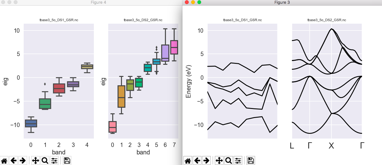
For further details about the AbiPy API and the GSR file, please consult the GsrFile notebook .