Parallelism on images, the string method
String method for the computation of minimum energy paths, in parallel.
This tutorial aims at showing how to use the parallelism on images, by performing a calculation of a minimum energy path (MEP) using the string method.
You will learn how to run the string method on a parallel architecture and what are the main input variables that govern convergence and numerical efficiency of the parallelism on images. Other algorithms use images, e.g. path-integral molecular dynamics, hyperdynamics, linear combination of images, … with different values of imgmov. The parallelism on images can be used for all these algorithms.
You are supposed to know already some basics of parallelism in ABINIT, explained in the tutorial A first introduction to ABINIT in parallel, and parallelism over bands and plane waves.
This tutorial should take about 1.5 hour and requires to have at least a 10 CPU core parallel computer.
Note
Supposing you made your own installation of ABINIT, the input files to run the examples are in the ~abinit/tests/ directory where ~abinit is the absolute path of the abinit top-level directory. If you have NOT made your own install, ask your system administrator where to find the package, especially the executable and test files.
In case you work on your own PC or workstation, to make things easier, we suggest you define some handy environment variables by executing the following lines in the terminal:
export ABI_HOME=Replace_with_absolute_path_to_abinit_top_level_dir # Change this line
export PATH=$ABI_HOME/src/98_main/:$PATH      # Do not change this line: path to executable
export ABI_TESTS=$ABI_HOME/tests/             # Do not change this line: path to tests dir
export ABI_PSPDIR=$ABI_TESTS/Pspdir/  # Do not change this line: path to pseudos dir
Examples in this tutorial use these shell variables: copy and paste
the code snippets into the terminal (remember to set ABI_HOME first!) or, alternatively,
source the set_abienv.sh script located in the ~abinit directory:
source ~abinit/set_abienv.sh
The ‘export PATH’ line adds the directory containing the executables to your PATH so that you can invoke the code by simply typing abinit in the terminal instead of providing the absolute path.
To execute the tutorials, create a working directory (Work*) and
copy there the input files of the lesson.
Most of the tutorials do not rely on parallelism (except specific tutorials on parallelism). However you can run most of the tutorial examples in parallel with MPI, see the topic on parallelism.
1 Summary of the String Method
The string method [Weinan2002] is an algorithm that allows the computation of a Minimum Energy Path (MEP) between an initial (i) and a final (f) configuration. It is inspired from the Nudge Elastic Band (NEB) method. A chain of configurations joining (i) to (f) is progressively driven to the MEP using an iterative procedure in which each iteration consists of two steps:
- Evolution step: the images are moved following the atomic forces.
- Reparametrization step: the images are equally redistributed along the string.
The algorithm presently implemented in ABINIT is the so-called simplified string method [Weinan2007]. It has been designed for the sampling of smooth energy landscapes.
Before continuing you might work in a different subdirectory as for the other tutorials. Why not work_paral_images?
Important
In what follows, the names of files are mentioned as if you were in this subdirectory.
All the input files can be found in the \$ABI_TESTS/tutoparal/Input directory.
You can compare your results with reference output files located in \$ABI_TESTS/tutoparal/Refs.
In the following, when “run ABINIT over nn CPU cores” appears, you have to use
a specific command line according to the operating system and architecture of
the computer you are using. This can be for instance: mpirun -n nn abinit input.abi
or the use of a specific submission file.
Tip
In this tutorial, most of the images and plots are easily obtained using the post-processing tool qAgate or agate, its core engine. Any post-process tool will work though !!
2 Computation of the initial and final configurations
We propose to compute the energy barrier for transferring a proton from an hydronium ion (H3O+) onto a NH3 molecule:
Starting from an hydronium ion and an ammoniac molecule, we obtain as final state a water molecule and an ammonium ion NH4+. In such a process, the MEP and the barrier are dependent on the distance between the hydronium ion and the NH3 molecule. Thus we choose to fix the O atom of H3O+ and the N atom of NH3 at a given distance from each other (4.0 Å = 7.5589 bohr). The calculation is performed using a LDA exchange-correlation functional.
You can visualize the initial and final states of the reaction below (H atoms are in white, the O atom is in red and the N atom in blue).

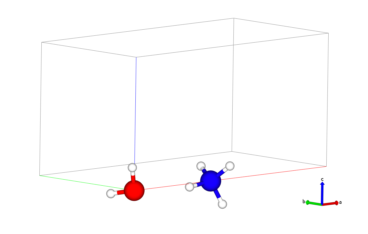
Tip
To obtain these images, open the timages_01.abi and timages_02.abi files with agate
or qAgate
Before using the string method, it is necessary to optimize the initial and
final points. The input files timages_01.abi and timages_02.abi contain
respectively two geometries close to the initial and final states of the
system. You have first to optimize properly these initial and final
configurations, using for instance the Broyden algorithm implemented in ABINIT.
#######################################
#       INPUT FILE FOR ABINIT         #
#                                     #
#  Hydronium ion + NH3 molecule       #
#  Ground state calculation           #
#  keeping O and H atoms fixed        #
#######################################

# Definition of the unit cell
# ===========================
natom         8

ntypat        3

# Species
#             O   N   H
znucl
              8   7   1

typat
              1   3   3   2   3   3   3   3

acell         1.90000000000000e+01   9.45000000000000e+00   9.45000000000000e+00

xcart
              0.00000000000000e+00   0.00000000000000e+00   0.00000000000000e+00 # O (H2O)
             -7.10348053351713e-01  -5.40272701392005e-01   1.64595146174340e+00 # H (H2O)
             -7.26410725481241e-01   1.63952639289158e+00  -5.39327838325563e-01 # H (H2O)
              7.55890453154257e+00   0.00000000000000e+00   0.00000000000000e+00 # N (NH3)
              8.21274977352101e+00  -1.88575770800658e-01  -1.80374359383935e+00 # H (NH3)
              8.16172716793309e+00  -1.48664754874114e+00   1.07147471734616e+00 # H (NH3)
              8.20330114285658e+00   1.65086474968890e+00   7.60236823259894e-01 # H (NH3)
              1.94263846460644e+00   4.28967832165041e-02   2.96309057636469e-02 # H (proton)

natfix        2
iatfix        1 4      # Keep O and N atoms fixed

pp_dirpath "$ABI_PSPDIR/"
pseudos "8o_hard.paw, 7n.paw, 1h.paw"

# Electronic configuration
# ========================
nband         10       # Number of bands to compute
kptopt        0        # No autogeneration of kpts so only use Gamma (0,0,0)
cellcharge    1.0      # Charge of the simulation cell

# Convergence parameters
# ======================
ecut          20
pawecutdg     40

# Control of the SCF cycle
# ========================
toldff        5.0d-7   # Stopping criterion of SCF cycle
nstep         50       # Maximal number of SCF steps

# Control of the relaxation
# =========================
geoopt        "bfgs"   # BFGS (Broyden) algorithm for ions relaxation
optcell       0        # No cell optimization
ntime         500      # Max. number of "time" steps
tolmxf        5.0d-5   # Stopping criterion of relaxation cycle

# Parallelization
# ===============
paral_kgb     1        # Force use of lobpcg WITH parallelism on 1 CPU
nblock_lobpcg 1


##############################################################
# This section is used only for regression testing of ABINIT #
##############################################################
#%%<BEGIN TEST_INFO>
#%% [setup]
#%% executable = abinit
#%% [files]
#%% [NCPU_1]
#%% files_to_test =
#%%   timages_01_MPI1.abo, tolnlines = 7, tolabs = 8.300e-05, tolrel = 2.500e-02, fld_options = -easy
#%% [paral_info]
#%% nprocs_to_test = 1
#%% max_nprocs = 1
#%% [extra_info]
#%% authors = G. Genestes, M. Torrent, J. Bieder
#%% keywords =
#%% description =
#%%   Hydronium ion + NH3 molecule
#%%   Ground state calculation
#%%   keeping O and H atoms fixed
#%%<END TEST_INFO>
#######################################
#       INPUT FILE FOR ABINIT         #
#                                     #
#  Hydronium ion + NH3 molecule       #
#  Ground state calculation           #
#  keeping O and H atoms fixed        #
#######################################

# Definition of the unit cell
# ===========================
natom         8

ntypat        3

# Species
#             O   N   H
znucl
              8   7   1

typat
              1   3   3   2   3   3   3   3

acell         1.90000000000000e+01   9.45000000000000e+00   9.45000000000000e+00

xcart
              0.00000000000000e+00   0.00000000000000e+00   0.00000000000000e+00 # O (H2O)
             -5.74665717010524e-01  -3.59803855701426e-01   1.71719413695318e+00 # H (H2O)
             -6.09436677855620e-01   1.70604475276916e+00  -3.55835430822367e-01 # H (H2O)
              7.55890453154257e+00   0.00000000000000e+00   0.00000000000000e+00 # N (NH3)
              8.47920115825788e+00  -2.81947139026538e-01  -1.69489536858513e+00 # H (NH3)
              7.96330592398010e+00  -1.48683652135442e+00   1.19222821723755e+00 # H (NH3)
              8.21841895191966e+00   1.64576248913011e+00   8.07291003968747e-01 # H (NH3)
              5.58603044880996e+00   1.05635690828307e-01  -2.56435836232582e-01 # H (proton)

natfix        2
iatfix        1 4      # Keep O and N atoms fixed

pp_dirpath "$ABI_PSPDIR/"
pseudos "8o_hard.paw, 7n.paw, 1h.paw"

# Electronic configuration
# ========================
nband         10       # Number of bands to compute
kptopt        0        # No autogeneration of kpts so only use Gamma (0,0,0)
cellcharge    1.0      # Charge of the simulation cell

# Convergence parameters
# ======================
ecut          20
pawecutdg     40

# Control of the SCF cycle
# ========================
toldff        5.0d-7   # Stopping criterion of SCF cycle
nstep         50       # Maximal number of SCF steps

# Control of the relaxation
# =========================
geoopt        "bfgs"   # BFGS (Broyden) algorithm for ions relaxation
optcell       0        # No cell optimization
ntime         500      # Max. number of "time" steps
tolmxf        5.0d-5   # Stopping criterion of relaxation cycle

# Parallelization
# ===============
paral_kgb     1        # Force use of lobpcg WITH parallelism on 1 CPU
nblock_lobpcg 1

#%%<BEGIN TEST_INFO>
#%% [setup]
#%% executable = abinit
#%% [files]
#%% [NCPU_1]
#%% files_to_test =
#%%   timages_02_MPI1.abo, tolnlines = 7, tolabs = 7.500e-04, tolrel = 2.100e-01, fld_options = -easy
#%% [paral_info]
#%% nprocs_to_test = 1
#%% max_nprocs = 1
#%% [extra_info]
#%% authors = G. Genestes, M. Torrent, J. Bieder
#%% keywords =
#%% description =
#%%   Hydronium ion + NH3 molecule
#%%   Ground state calculation
#%%   keeping O and H atoms fixed
#%%<END TEST_INFO>
Open the timages_01.abi file and look at it carefully. The unit cell is defined
at the begining. Note that the keywords natfix and iatfix are used to keep
fixed the positions of the O and N atoms. The cell is tetragonal and its size
is larger along x so that the periodic images of the system are separated by
4.0 Å (7.5589 bohr) of vacuum in the three directions. The keyword cellcharge is used to
remove an electron of the system and thus obtain a protonated molecule
(neutrality is recovered by adding a uniform compensating charge background).
Although this input file will run on a single core, the paral_kgb keyword is set to 1 to activate the LOBPCG [Bottin2008] algorithm.
Important
If your system were larger and required more CPU time, all the usual variables for parallelism np_spkpt, npband, npfft, npspinor could be used wisely.
Then run the calculation in sequential, first for the initial
configuration (timages_01.abi), and then for the final one (timages_02.abi). You
should obtain the following positions:
-
for the initial configuration:
xcart 0.0000000000E+00 0.0000000000E+00 0.0000000000E+00 -7.1119330966E-01 -5.3954252784E-01 1.6461078895E+00 -7.2706367116E-01 1.6395559231E+00 -5.3864186404E-01 7.5589045315E+00 0.0000000000E+00 0.0000000000E+00 8.2134747935E+00 -1.8873337293E-01 -1.8040045499E+00 8.1621251369E+00 -1.4868515614E+00 1.0711027413E+00 8.2046046694E+00 1.6513534511E+00 7.5956562273E-01 1.9429112745E+00 4.2303909125E-02 2.9000318893E-02 -
for the final configuration:
xcart      0.0000000000E+00  0.0000000000E+00  0.0000000000E+00
          -5.8991482730E-01 -3.6948430331E-01  1.7099330811E+00
          -6.3146217793E-01  1.6964706443E+00 -3.6340264832E-01
           7.5589045315E+00  0.0000000000E+00  0.0000000000E+00
           8.4775515860E+00 -2.9286989031E-01 -1.6949564152E+00
           7.9555913454E+00 -1.4851844626E+00  1.1974660442E+00
           8.2294855730E+00  1.6454040992E+00  8.0048724879E-01
           5.5879660323E+00  1.1438061815E-01 -2.5524007156E-01
3 Related keywords
Once you have properly optimized the initial and final states of the process, you can turn to the computation of the MEP. Let us first have a look at the related keywords.
- imgmov
-
Selects an algorithm using replicas of the unit cell. For the string method, choose 2.
- nimage
-
gives the number of replicas of the unit cell including the initial and final ones. Note that when nimage>1, the default value of several print input variables changes from one to zero. You might want to explicitly set prtgsr to 1 to print the _GSR file, and get some visualization possibilities using Abipy.
- dynimage(nimage)
-
arrays of flags specifying if the image evolves or not (0: does not evolve; 1: evolves).
- ntimimage
-
gives the maximum number of iterations (for the relaxation of the string).
- tolimg
-
convergence criterion (in Hartree) on the total energy (averaged over the nimage images).
- fxcartfactor
-
“time step” (in Bohr2/Hartree) for the evolution step of the string method. For the time being (ABINITv6.10), only steepest-descent algorithm is implemented.
- npimage
-
gives the number of processors among which the work load over the image level is shared. Only dynamical images are considered (images for which dynimage is 1). This input variable can be automatically set by ABINIT if the number of processors is large enough.
- prtvolimg
-
governs the printing volume in the output file (0: full output; 1: intermediate; 2: minimum output).
4 Computation of the MEP without parallelism over images
You can now start with the string method. First, for test purpose, we will not use the parallelism over images and will thus only perform one step of string method.
#######################################
#       INPUT FILE FOR ABINIT         #
#                                     #
#  Hydronium ion + NH3 molecule       #
#  String method                      #
#  Moving the proton from H2O to NH3  #
#  keeping O and H atoms fixed        #
#######################################

# Definition of the unit cell
# ===========================
natom         8

ntypat        3

# Species
#             O   N   H
znucl
              8   7   1

typat
              1   3   3   2   3   3   3   3

acell         1.90000000000000e+01   9.45000000000000e+00   9.45000000000000e+00

natfix        2
iatfix        1 4

pp_dirpath "$ABI_PSPDIR/"
pseudos "8o_hard.paw, 7n.paw, 1h.paw"

# Electronic configuration
# ========================
nband         10       # Number of bands to compute
kptopt        0        # No autogeneration of kpts so only use Gamma (0,0,0)
cellcharge    1.0      # Charge of the simulation cell

# Convergence parameters
# ======================
ecut          20
pawecutdg     40

# Control of the SCF cycle
# ========================
toldff        5.0d-7   # Stopping criterion of SCF cycle
nstep         50       # Maximal number of SCF steps

# Parallelization
# ===============
paral_kgb     1        # Force use of lobpcg WITH parallelism on 1 CPU
nblock_lobpcg 1

# Definition of the path
# ======================
xcart
              0.00000000000000e+00   0.00000000000000e+00   0.00000000000000e+00
             -7.11193309720352e-01  -5.39542527497972e-01   1.64610788936525e+00
             -7.27063671207315e-01   1.63955592306938e+00  -5.38641863769265e-01
              7.55890453154257e+00   0.00000000000000e+00   0.00000000000000e+00
              8.21347479352361e+00  -1.88733372964621e-01  -1.80400454958594e+00
              8.16212513700922e+00  -1.48685156144099e+00   1.07110274118997e+00
              8.20460466973224e+00   1.65135345075879e+00   7.59565622295564e-01
              1.94291127433874e+00   4.23039089066905e-02   2.90003186750848e-02


xcart_lastimg
              0.00000000000000e+00   0.00000000000000e+00   0.00000000000000e+00
             -5.89914827008103e-01  -3.69484303034365e-01   1.70993308126728e+00
             -6.31462177443216e-01   1.69647064450604e+00  -3.63402648099217e-01
              7.55890453154257e+00   0.00000000000000e+00   0.00000000000000e+00
              8.47755158608181e+00  -2.92869889937304e-01  -1.69495641512467e+00
              7.95559134567592e+00  -1.48518446265367e+00   1.19746604398273e+00
              8.22948557282829e+00   1.64540409916636e+00   8.00487248896275e-01
              5.58796603232530e+00   1.14380617889722e-01  -2.55240071529671e-01


# String controls
# ===============
nimage        12         # Number of points along the string
imgmov        2          # Selection of "String Method" algo
ntimimage     1          # Max. number of relaxation steps of the string
tolimg        0.0001     # Tol. criterion (will stop when average energy of cells < tolimg)
dynimage      0 10*1 0   # Keep first and last images fixed


#%%<BEGIN TEST_INFO>
#%% [setup]
#%% executable = abinit
#%% [files]
#%% [NCPU_1]
#%% files_to_test =
#%%   timages_03_MPI1.abo, tolnlines = 82, tolabs = 3.200e-04, tolrel = 1.500e-01, fld_options = -easy
#%% [paral_info]
#%% nprocs_to_test = 1
#%% max_nprocs = 1
#%% [extra_info]
#%% description =
#%%   Hydronium ion + NH3 molecule
#%%   String method
#%%   Moving the proton from H2O to NH3
#%%   keeping O and H atoms fixed
#%%<END TEST_INFO>
Open the timages_03.abi file and look at it. The initial and final
configurations are specified at the end through the keywords xcart and
xcart_lastimg. By default, ABINIT generates the intermediate
images by a linear interpolation between these two configurations. In this
first calculation, we will sample the MEP with 12 points (2 are fixed and
correspond to the initial and final states, 10 are evolving). nimage is
thus set to 12. The npimage variable is not used yet (no parallelism over
images) and ntimimage is set to 1 (only one time step).
Since the parallelism over the images is not used, this calculation still runs over 1 CPU core.
5 Computation of the MEP using parallelism over images
Now you can perform the complete computation of the MEP using the parallelism over the images.
#######################################
#       INPUT FILE FOR ABINIT         #
#                                     #
#  Hydronium ion + NH3 molecule       #
#  String method                      #
#  Moving the proton from H2O to NH3  #
#  keeping O and H atoms fixed        #
#######################################

# Definition of the unit cell
# ===========================
natom         8

ntypat        3

# Species
#             O   N   H
znucl
              8   7   1

typat
              1   3   3   2   3   3   3   3

acell         1.90000000000000e+01   9.45000000000000e+00   9.45000000000000e+00

natfix        2
iatfix        1 4

pp_dirpath "$ABI_PSPDIR/"
pseudos "8o_hard.paw, 7n.paw, 1h.paw"

# Electronic configuration
# ========================
nband         10       # Number of bands to compute
kptopt        0        # No autogeneration of kpts so only use Gamma (0,0,0)
cellcharge    1.0      # Charge of the simulation cell

# Convergence parameters
# ======================
ecut          20
pawecutdg     40

# Control of the SCF cycle
# ========================
# In order to obtain portability of the test, a much too stringent value for toldff is asked, and the limitation of the number of steps
# is governed by a relatively low nstep. In real production conditions, the commented values would be better.
toldff        1.0d-9 # 5.0d-7   # Stopping criterion of SCF cycle
nstep         12     #   50       # Maximal number of SCF steps

# Parallelization
# ===============
paral_kgb     1        # Force use of lobpcg WITH parallelism on 1 CPU
nblock_lobpcg 1
npimage       10       # Use 10 CPUs for the image parallelization

# Definition of the path
# ======================
xcart
              0.00000000000000e+00   0.00000000000000e+00   0.00000000000000e+00
             -7.11193309720352e-01  -5.39542527497972e-01   1.64610788936525e+00
             -7.27063671207315e-01   1.63955592306938e+00  -5.38641863769265e-01
              7.55890453154257e+00   0.00000000000000e+00   0.00000000000000e+00
              8.21347479352361e+00  -1.88733372964621e-01  -1.80400454958594e+00
              8.16212513700922e+00  -1.48685156144099e+00   1.07110274118997e+00
              8.20460466973224e+00   1.65135345075879e+00   7.59565622295564e-01
              1.94291127433874e+00   4.23039089066905e-02   2.90003186750848e-02


xcart_lastimg
              0.00000000000000e+00   0.00000000000000e+00   0.00000000000000e+00
             -5.89914827008103e-01  -3.69484303034365e-01   1.70993308126728e+00
             -6.31462177443216e-01   1.69647064450604e+00  -3.63402648099217e-01
              7.55890453154257e+00   0.00000000000000e+00   0.00000000000000e+00
              8.47755158608181e+00  -2.92869889937304e-01  -1.69495641512467e+00
              7.95559134567592e+00  -1.48518446265367e+00   1.19746604398273e+00
              8.22948557282829e+00   1.64540409916636e+00   8.00487248896275e-01
              5.58796603232530e+00   1.14380617889722e-01  -2.55240071529671e-01


# String controls
# ===============
nimage        12         # Number of points along the string
imgmov        2          # Selection of "String Method" algo
ntimimage     50         # Max. number of relaxation steps of the string
tolimg        0.0001     # Tol. criterion (will stop when average energy of cells < tolimg)
dynimage      0 10*1 0   # Keep first and last images fixed


#%%<BEGIN TEST_INFO>
#%% [setup]
#%% executable = abinit
#%% exclude_builders = scope_gnu_12.2_mpich
#%% [files]
#%% [NCPU_10]
#%% files_to_test =
#%%   timages_04_MPI10.abo, tolnlines = 55, tolabs = 5.5e-3, tolrel = 9.3e-1, fld_options = -easy;
#%% [paral_info]
#%% nprocs_to_test = 10
#%% max_nprocs = 10
#%% [extra_info]
#%% description =
#%%   Hydronium ion + NH3 molecule
#%%   String method
#%%   Moving the proton from H2O to NH3
#%%   keeping O and H atoms fixed
#%%<END TEST_INFO>
Open the timages_04.abi file. The keyword npimage has been added and set to 10, and
ntimimage has been increased to 50.
This calculation has thus to be run over 10 CPU cores.
The convergence of the string method algorithm is controlled by tolimg, which has been set to 0.0001 Ha. In order to obtain a more lisible output file, you can decrease the printing volume and set prtvolimg to 2. Then run ABINIT over 10 CPU cores.
When the calculation is completed, ABINIT provides you with 12 configurations that sample the Minimum Energy Path between the initial (i) and final (f) states. Plotting the total energy of these configurations with respect to a reaction coordinate that join (i) to (f) gives you the energy barrier that separates (i) from (f). In our case, a natural reaction coordinate can be the distance between the hopping proton and the O atom of H2O (dOH), or equivalently the distance between the proton and the N atom (dHN). The graph below shows the total energy as a function of the OH distance along the MEP. It indicates that the barrier for crossing from H2O to NH3 is ~1.36 eV. The 6th image gives an approximate geometry of the transition state. Note that in the initial state, the OH distance is significantly stretched, due to the presence of the NH3 molecule.
Tip
Note that the total energy of each of the 12 replicas of the simulation cell can be found at the end of the output file in the section:
-outvars: echo values of variables after computation --------
Tip
Also, you can can have a look at the atomic positions in each image: in cartesian coordinates (xcart_1img, xcart_2img, …) or in reduced coordinates (xred_1img, xred_2img, …) to compute the OH distance.
Tip
You can issue the command :plot xy x="distance 1 8 dunit=A" y="etotal eunit=eV" in agate or qAgate
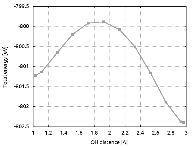
Total energy as a function of OH distance for the path computed with 12 images
and tolimg=0.0001 (which is very close to the x coordinate of the proton: first coordinate of xcart for the 8th atom in the output file).
The keyword npimage can be automatically set by ABINIT if autoparal is set to 1.
Let us test this functionality. Edit again the timages_04.abi file and comment
the npimage line, then add autoparal=1. Then run the calculation again over 10 CPU cores.
Open the output file and look at the npimage value …
6 Converging the MEP
Like all physical quantities, the MEP has to be converged with respect to some numerical parameters. The two most important are the number of points along the path (nimage) and the convergence criterion (tolimg).
-
Increase the number of images to 22 (2 fixed + 20 evolving) and recompute the MEP. Don’t forget to update dynimage to
0 20*1 0! And you have 20 CPU cores available then set npimage to 20 and run ABINIT over 20 CPU cores. The graph below superimposes the previous MEP (grey curve, calculated with 12 images) and the new one obtained by using 22 images (cyan curve). You can see that the global profile is almost not modified as well as the energy barrier.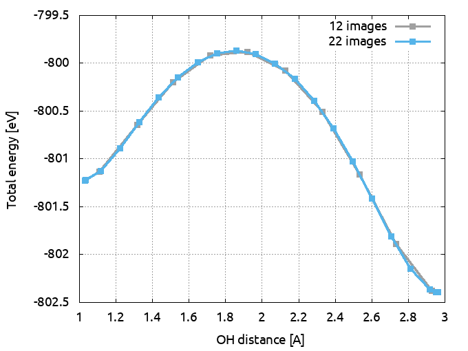
Total energy as a function of OH distance for the path computed with 12 images and tolimg=0.0001 (grey curve) and the one computed with 22 images and tolimg=0.0001 (red curve).
Tip
The image can be obtained with
agateorqagatewith the following commandsReplace:open timages_04_MPI10o_HIST.nc # 12 images calculation :plot xy x="distance 1 8 dunit=A" y="etotal eunit=eV" hold=true :open timages_04_MPI10_22o_HIST.nc # 22 images calculation :plot xy x="distance 1 8 dunit=A" y="etotal eunit=eV"plotwithprintto get thegnuplotscript.The following animation is made by putting together the 22 images obtained at the end of this calculation, from (i) to (f) and then from (f) to (i). It allows to visualize the MEP.
Tip
Open the
timages_04o_HIST.ncfile withagateorqAgateto produce this animation.
-
Come back to nimage=12. First you can increase tolimg to 0.001 and recompute the MEP. This will be much faster than in the previous case.
Then you should decrease tolimg to 0.00001 and recompute the MEP. To gain CPU time, you can start your calculation by using the 12 images obtained at the end of the calculation that used tolimg = 0.0001. In your input file, these starting images will be specified by the keywords xcart, xcart_2img, xcart_3img … xcart_12img. You can copy them directly from the output file obtained at the previous section. The graph below superimposes the path obtained with 12 images and tolimg=0.001 (grey curve) and the one with 12 images and tolimg=0.0001 (cyan curve).
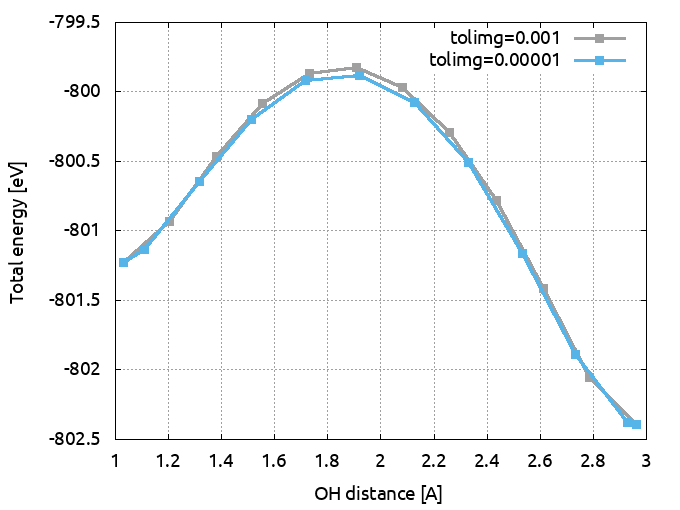
Total energy as a function of OH distance for the path computed with 12 images and tolimg=0.0001 (cyan curve) and the one computed with 12 images and tolimg=0.001 (grey curve).