Static non-linear properties
Electronic non-linear susceptibility, non-resonant Raman tensor, electro-optic effect.
This tutorial shows how to obtain the following non-linear physical properties, for an insulator:
- The non-linear optical susceptibilities
- The Raman tensor of TO and LO modes
- The electro-optic coefficients
We will study the compound AlP. During the preliminary steps needed to compute non-linear properties, we will also obtain several linear response properties:
- The Born effective charges
- The dielectric constant
- The proper piezoelectric tensor (clamped and relaxed ions)
Finally, we will also compute the derivative of the susceptibility tensor with respect to atomic positions (Raman tensor), using finite differences.
The user should have already completed several advanced tutorials, including: Response-Function 1, Response-Function 2, Polarization and Finite electric fields, and the Elastic properties.
This tutorial should take about 1 hour and 30 minutes.
Note
Supposing you made your own installation of ABINIT, the input files to run the examples are in the ~abinit/tests/ directory where ~abinit is the absolute path of the abinit top-level directory. If you have NOT made your own install, ask your system administrator where to find the package, especially the executable and test files.
In case you work on your own PC or workstation, to make things easier, we suggest you define some handy environment variables by executing the following lines in the terminal:
export ABI_HOME=Replace_with_absolute_path_to_abinit_top_level_dir # Change this line
export PATH=$ABI_HOME/src/98_main/:$PATH      # Do not change this line: path to executable
export ABI_TESTS=$ABI_HOME/tests/             # Do not change this line: path to tests dir
export ABI_PSPDIR=$ABI_TESTS/Pspdir/  # Do not change this line: path to pseudos dir
Examples in this tutorial use these shell variables: copy and paste
the code snippets into the terminal (remember to set ABI_HOME first!) or, alternatively,
source the set_abienv.sh script located in the ~abinit directory:
source ~abinit/set_abienv.sh
The ‘export PATH’ line adds the directory containing the executables to your PATH so that you can invoke the code by simply typing abinit in the terminal instead of providing the absolute path.
To execute the tutorials, create a working directory (Work*) and
copy there the input files of the lesson.
Most of the tutorials do not rely on parallelism (except specific tutorials on parallelism). However you can run most of the tutorial examples in parallel with MPI, see the topic on parallelism.
1 Ground-state properties of AlP and general parameters
Before beginning, you might consider working in a different subdirectory, as for the other tutorials. For example, create Work_NLO in $ABI_TESTS/tutorespfn/Input.
In order to save some time, you might immediately start running a calculation.
Copy the file tnlo_2.abi from $ABI_TESTS/tutorespfn/Input to Work_NLO.
Run abinit on this file; it will take several minutes on a desktop PC.
In this tutorial we will assume that the ground-state properties of AlP have been previously obtained, and that the corresponding convergence studies have been done. Let us emphasize that, from our experience, accurate and trustable results for third order energy derivatives usually require a extremely high level of convergence. So, even if it is not always very apparent here, careful convergence studies must be explicitly performed in any practical study you attempt after this tutorial. As usual, convergence tests must be done on the property of interest (thus it is insufficient to determine parameters giving proper convergence only on the total energy, and to use them blindly for non-linear properties).
We will adopt the following set of generic parameters (quite similar to those in the tutorial on Polarization and finite electric field):
acell   3*7.1391127387E+00
rprim      0.0000000000E+00  7.0710678119E-01  7.0710678119E-01
           7.0710678119E-01  0.0000000000E+00  7.0710678119E-01
           7.0710678119E-01  7.0710678119E-01  0.0000000000E+00
ecut    2.8
ecutsm  0.5
dilatmx 1.05
nband   4 (=number of occupied bands)
ngkpt   6 6 6
nshiftk 4
shiftk  0.5 0.5 0.5
        0.5 0.0 0.0
        0.0 0.5 0.0
        0.0 0.0 0.5

pseudopotentials  Pseudodojo_nc_sr_04_pw_standard_psp8/P.psp8
                  Pseudodojo_nc_sr_04_pw_standard_psp8/Al.psp8
In principle, the acell to be used should be the one corresponding to the optimized structure at the ecut, and ngkpt combined with nshiftk and shiftk, chosen for the calculations. Unfortunately, for the purpose of this tutorial, in order to limit the duration of the runs, we have to work at an unusually low cutoff of 2.8 Ha for which the optimized lattice constant is unrealistic and equal to 7.139 Bohr (instead of the converged value of 7.251). In what follows, the lattice constant has been arbitrarily fixed to 7.139. Bohr. For comparison, results with ecut = 5 and 30 are also reported and, in those cases, were obtained at the optimized lattice constants of 7.273 and 7.251 Bohr. For those who would like to try later, convergence tests and structural optimizations can be done using the file $ABI_TESTS/tutorespfn/Input/tnlo_1.abi.
#Structural optimisation

#ndtset 6    jdtset 1 2 3 4 5 6

#  ngkpt1  6  6  6
#  ngkpt2  8  8  8
#  ngkpt3 10 10 10
#  ngkpt4 12 12 12
#  ngkpt5 14 14 14
#  ngkpt6 16 16 16

  ngkpt  6  6  6   # In the present example, only this grid of k points is considered
                   # A full convergence study on k points should be done, see the above lines.

#Definition of the unit cell
#**********************************
acell 3*10.53
rprim
0 1/2 1/2
1/2 0 1/2
1/2 1/2 0

#Definition of the atom types and pseudopotentials
 ntypat 2 # two types of atoms
 znucl 15 13 # the atom types are Phosphorous and Aluminum

# the following norm-conserving pseudopotentials are stored in the abinit distribution, but are freely
# available through www.pseudo-dojo.org
# this set uses the Perdew-Wang parameterization of LDA for the xc model
 pp_dirpath "$ABI_PSPDIR"
 pseudos "Psdj_nc_sr_04_pw_std_psp8/P.psp8, Psdj_nc_sr_04_pw_std_psp8/Al.psp8"

#Definition of the atoms
 natom 2 # two atoms in the cell
 typat 1 2 # type 1 is Phosphorous, type 2 is Aluminum (order defined by znucl above and pseudos list)
 nband 4 # nband is restricted here to the number of filled bands only, no empty bands.
 nbdbuf 0

# atomic positions in units of cell vectors
xred
1/4 1/4 1/4
0 0 0

#Numerical parameters of the calculation : planewave basis set and k point grid
ecut  2.8 # this value is very low but is used here to achieve very low calculation times.
        # in a production environment this should be checked carefully for convergence and
        # a more reasonable value is probably around 30
ecutsm 0.5
dilatmx 1.05
nshiftk 4 # this Monkhorst-Pack shift pattern is used so that the symmetry of the shifted grid
          # is correct. A gamma-centered grid would also have the correct symmetry but would be
          # less efficient.
shiftk 0.5 0.5 0.5
       0.5 0.0 0.0
       0.0 0.5 0.0
       0.0 0.0 0.5

# scf parameters
nstep 8  # limit number of steps for the tutorial, in general this should be set to its
         # default (30) or higher

# suppress printing of density, wavefunctions, etc except what is
# explicitly requested above in the ndtset section
prtwf 0
prtden 0
prteig 0

#Structural relaxation
#*********************
   geoopt "bfgs"
   optcell 2
   tolvrs 1.0d-15
   tolmxf 5.0d-6
   ntime 100

##############################################################
# This section is used only for regression testing of ABINIT #
##############################################################
#%%<BEGIN TEST_INFO>
#%% [setup]
#%% executable = abinit
#%% [files]
#%% files_to_test =
#%%   tnlo_1.abo, tolnlines=  1, tolabs=  4.192e-06, tolrel=  8.000e-05, fld_options=-medium
#%% [paral_info]
#%% max_nprocs = 2
#%% [extra_info]
#%% authors = J. Zwanziger, M. Veithen, P. Ghosez
#%% keywords =
#%% description = Structural optimisation
#%%<END TEST_INFO>
Before going further, you might refresh your memory concerning the other variables: ecutsm, dilatmx, and nbdbuf.
2 Linear and non-linear responses from density functional perturbation theory (DFPT)
As a theoretical support to this section of the tutorial, you might consider reading [Veithen2005].
In the first part of this tutorial, we will describe how to compute various linear and non-linear responses directly connected to second-order and third- order derivatives of the energy, using DFPT. From the \((2n+1)\) theorem, computation of energy derivatives up to third order only requires the knowledge of the ground-state and first-order wavefunctions, see [Gonze1989] and [Gonze1995]. Our study will therefore include the following steps : (i) computation of the ground-state wavefunctions and density; (ii) determination of wavefunctions derivatives and construction of the related databases for second and third- order energy derivatives, (iii) combination of the different databases and analysis to get the physical properties of interest.
These steps are closely related to what was done for the dielectric and dynamical properties, except that an additional database for third-order energy derivatives will now be computed during the run. Only selected third-order derivatives are implemented at present in ABINIT, and concern responses to electric field and atomic displacements:
-
non-linear optical susceptibilities (related to a third-order derivative of the energy with respect to electric fields at clamped nuclei positions)
-
Raman susceptibilities (mixed third-order derivative of the energy, twice with respect to electric fields at clamped nuclei positions, and once with respect to atomic displacement)
-
Electro-optic coefficients (related to a third-order derivative of the energy with respect to electric fields, two of them being optical fields, that is, for clamped ionic positions, and one of them being a static field, for which the ionic positions are allowed to relax)
The various steps are combined into a single input file.
There are two implementations available in ABINIT for the computation of third-order derivatives which includes at least one electric field perturbation (so all tensors mentioned above). First we will present the PEAD method, as described in [Veithen2005], then we will present the full DFPT method, as described in [Gonze2020] and [Romero2020]. In the latter case, the input file is slightly modified so the reader interested in full DFPT should read the PEAD part first. Only the full DFPT implementation is available for PAW pseudopotentials.
Responses to electric fields, atomic displacements, and strains (with PEAD)
Let us examine the file tnlo_2.abi.
# Linear and nonlinear response calculation for AlP
# Perturbations: electric fields & atomic displacements

ndtset 5

#DATASET1 : scf calculation: GS WF in the IBZ
#********************************************
   prtden1    1        # save density on disk, will be used in other datasets
    prtwf1    1        # save WF on disk, will be used in other datasets
   kptopt1    1        # use Irreducible Brillouin Zone (all symmetry taken into account)
   toldfe1    1.0d-12  # SCF convergence criteria (could be tolwfr or tolvrs)

#DATASET2 : non scf calculation: GS WF in half BZ
#*****************************************************
   getden2    1        # use density from dataset 1
   kptopt2    2        # use Half Brillouin Zone (only time-reversal symmetry taken into account)
   getwfk2    1        # use GS WF from dataset 1 (as input)
     iscf2   -2        # non-self-consistent calculation
   tolwfr2    1.0d-22  # convergence criteria on WF, need high precision for response
    prtwf2    1        # save WF on disk, will be used in other datasets

#DATASET3 : derivative of WF with respect to k points (d/dk)
#**********************************************************
   getwfk3    2        # use GS WF from dataset 2
   kptopt3    2        # use Half Brillouin Zone (only time-reversal symmetry taken into account)
   rfelfd3    2        # compute 1st-order WF derivatives (d/dk)
   tolwfr3    1.0d-22  # convergence criteria on 1st-order WF
    prtwf3    1        # save 1st-order WF on disk, will be used in other datasets

#DATASET4 : response functions (2nd derivatives of E)
#           and corresponding 1st order WF derivatives
#           phonons, electric fields, and strains are all done
#**************************************************************
   getwfk4    2        # use GS WF from dataset 2
   kptopt4    2        # use Half Brillouin Zone (only time-reversal symmetry taken into account)
   getddk4    3        # use ddk WF from dataset 3 (needed for electric field)
   rfphon4    1        # compute 1st-order WF derivatives with respect to atomic displacements...
   rfelfd4    3        # compute 1st-order WF derivatives with respect to electric field
   rfstrs4    3        # compute 1st-order WF derivatives with respect to strains
   tolvrs4    1.0d-12  # SCF convergence criteria (could be tolwfr)
  prepanl4    1        # make sure that response functions are correctly prepared for a non-linear computation
    prtwf4    1        # save 1st-order WF on disk, will be used in other datasets
   prtden4    1        # save 1st-order density on disk, will be used in other datasets

#DATASET5 : 3rd derivatives of E
#*********************************
   getwfk5           2     # use GS WF from dataset 2
  get1den5           4     # use 1st-order densities from dataset 4
   get1wf5           4     # use 1st-order WFs from dataset 4
   kptopt5           2     # use Half Brillouin Zone (only time-reversal symmetry taken into account)
optdriver5           5     # compute 3rd order derivatives of the energy
  d3e_pert1_elfd5    1     # activate electric field for 1st perturbation...
  d3e_pert1_phon5    1     # ...and also atomic displacements...
 d3e_pert1_atpol5    1 2   # ...for all atoms (so here only 1 and 2)...
  d3e_pert2_elfd5    1     # activate electric field for 2nd perturbation...
  d3e_pert3_elfd5    1     # activate electric field for 3rd perturbation...

#Definition of the unit cell
# these cell parameters were derived from a relaxation run done with the
# current ecut and kpt values. The current ecut value used is very low but
# is done to speed the calculations.
# acell      7.2728565836E+00  7.2728565836E+00  7.2728565836E+00 Bohr # ecut 5
# acell      7.2511099467E+00  7.2511099467E+00  7.2511099467E+00 Bohr # ecut 30
acell      7.1391127387E+00  7.1391127387E+00  7.1391127387E+00 Bohr # ecut 2.8
rprim      0.0000000000E+00  7.0710678119E-01  7.0710678119E-01
           7.0710678119E-01  0.0000000000E+00  7.0710678119E-01
           7.0710678119E-01  7.0710678119E-01  0.0000000000E+00

#Definition of the atom types and pseudopotentials
 ntypat 2 # two types of atoms
 znucl 15 13 # the atom types are Phosphorous and Aluminum

# the following norm-conserving pseudopotentials are stored in the abinit distribution, but are freely
# available through www.pseudo-dojo.org
# this set uses the Perdew-Wang parameterization of LDA for the xc model
 pp_dirpath "$ABI_PSPDIR"
 pseudos "Psdj_nc_sr_04_pw_std_psp8/P.psp8, Psdj_nc_sr_04_pw_std_psp8/Al.psp8"

#Definition of the atoms
 natom 2 # two atoms in the cell
 typat 1 2 # type 1 is Phosphorous, type 2 is Aluminum (order defined by znucl above and pseudos list)
 nband 4 # nband is restricted here to the number of filled bands only, no empty bands.
 nbdbuf 0

# atomic positions in units of cell vectors
xred
1/4 1/4 1/4
0 0 0

#Numerical parameters of the calculation : planewave basis set and k point grid
ecut  2.8 # this value is very low but is used here to achieve very low calculation times.
        # in a production environment this should be checked carefully for convergence and
        # a more reasonable value is probably around 30
ecutsm 0.5
ngkpt 6 6 6 # must be checked carefully for convergence, Raman calculations converge slowly with kpt
nshiftk 4 # this Monkhorst-Pack shift pattern is used so that the symmetry of the shifted grid
          # is correct. A gamma-centered grid would also have the correct symmetry but would be
          # less efficient.
shiftk 0.5 0.5 0.5
       0.5 0.0 0.0
       0.0 0.5 0.0
       0.0 0.0 0.5

# scf parameters
nstep 8  # limit number of steps for the tutorial, in general this should be set to its
         # default (30) or higher

# suppress printing of density, wavefunctions, etc except what is
# explicitly requested above in the ndtset section
prtwf 0
prtden 0
prteig 0

##############################################################
# This section is used only for regression testing of ABINIT #
##############################################################
#%%<BEGIN TEST_INFO>
#%% [setup]
#%% executable = abinit
#%% test_chain = tnlo_2.abi, tnlo_3.abi, tnlo_4.abi
#%% [files]
#%% files_to_test =
#%%   tnlo_2.abo, tolnlines=7 , tolabs=  2.000e-04, tolrel=  4.000e-02, fld_options=-medium
#%% [paral_info]
#%% max_nprocs = 2
#%% [extra_info]
#%% authors =  J. Zwanziger, L. Baguet, M. Veithen
#%% keywords = NC, DFPT, NONLINEAR
#%% description =
#%%   Linear and nonlinear response calculation for AlP
#%%   Perturbations: electric fields & atomic displacements
#%%<END TEST_INFO>
Its purpose is to build databases for second and third energy derivatives with respect to electric fields, atomic displacements, and strains. You can edit it. It is made of 5 datasets. The first four data sets are nearly the same as for a typical linear response calculation: (1) a self-consistent calculation of the ground state in the irreducible Brillouin Zone; (2) non self-consistent calculation of the ground state to get the wavefunctions over the full Brillouin Zone; (3) Computation of the derivatives of the wavefunctions with respect to k points, using DFPT; (4) second derivatives of the energy and related first-order wavefunctions with respect to electric field, atomic displacements, and strains; and finally (5) the third derivative calculations. Some specific features must however be explicitly specified in order to prepare for the non-linear response step (dataset 5). First, it is mandatory to specify:
nbdbuf  0
nband   4 (= number of valence bands)
prtden4    1
prepanl4   1
Note also that while the strain perturbation is not used in dataset 5, the information it provides is necessary to obtain some of the relaxed ion properties that will be examined later.
The input to dataset 5 trigger the various third-order derivatives to be computed. This section includes the following:
   getwfk5    2
  get1den5    4
   get1wf5    4
   kptopt5    2
optdriver5    5
  d3e_pert1_elfd5    1
  d3e_pert1_phon5    1
 d3e_pert1_atpol5    1 2
  d3e_pert2_elfd5    1
  d3e_pert3_elfd5    1
The d3e input
variables determine the 3 perturbations of the 3rd order derivatives, and their
directions. Notice that we compute three derivatives with respect to electric field:
d3e_pert1_elfd, d3e_pert2_elfd, and d3e_pert3_elfd. These will be combined
to give the necessary data for the nonlinear optical susceptibility. We also
include d3e_pert1_phon, for both atoms in the unit cell (see d3e_pert1_atpol, for which we stick to the default).
When combined
later with the electric field perturbations 2 and 3, this will yield the necessary
information for the Raman tensor. Finally, for all three perturbation classes, we compute
the perturbations in all three spatial directions
(see d3e_pert1_dir, d3e_pert2_dir and d3e_pert3_dir, for which we stick to the default).
If it was not done at the beginning of this tutorial, you can now make the run. You can have a quick look to the output file to verify that everything is OK. It contains the values of second and third energy derivatives. It has however no immediate interest since the information is not presented in a very convenient format. The relevant information is in fact also stored in the database files (DDB) generated independently for second and third energy derivatives at the end of run steps 4 and 5. Keep these databases, as they will be used later for a global and convenient analysis of the results using ANADDB.
Responses to electric fields, atomic displacements, and strains (with full DFPT)
If not already done, the reader should read the part on the PEAD method.
Contrary to PEAD, with full DFPT the electric field is treated analytically, the same way it is done for the computation of second-order derivatives of the energy (see Response-Function 1). One needs first order wavefunctions derivatives with respect to k-points (dataset 3 of tnlo_2.abi). to compute second order energy derivatives with an electric field perturbation (dataset 4 of tnlo_2.abi). It turns out that third-order derivatives of the energy, in this context, needs second derivatives of wavefunctions with respect to electric fields and k-points. To compute the latter one also needs second derivatives of wavefunctions with respect to k-points only, so in total we need two additional sets of wavefunctions derivatives.
Now you can compare the files tnlo_2.abi and tnlo_6.abi.
# Linear and nonlinear response calculation for AlP
# Perturbations: electric fields & atomic displacements
# Use of 'full DFPT' method for third derivatives,
# so we need to solve Second Order Sternheimer equation

ndtset 7

#DATASET1 : scf calculation: GS WF in the IBZ
#********************************************
   prtden1    1        # save density on disk, will be used in other datasets
    prtwf1    1        # save WF on disk, will be used in other datasets
   kptopt1    1        # use Irreducible Brillouin Zone (all symmetry taken into account)
   toldfe1    1.0d-12  # SCF convergence criteria (could be tolwfr or tolvrs)

#DATASET2 : non scf calculation: GS WF in half BZ
#*****************************************************
   getden2    1        # use density from dataset 1
   kptopt2    2        # use Half Brillouin Zone (only time-reversal symmetry taken into account)
   getwfk2    1        # use GS WF from dataset 1 (as input)
     iscf2   -2        # non-self-consistent calculation
   tolwfr2    1.0d-22  # convergence criteria on WF, need high precision for response
    prtwf2    1        # save WF on disk, will be used in other datasets

#DATASET3 : derivative of WF with respect to k points (d/dk)
#**********************************************************
   getwfk3    2        # use GS WF from dataset 2
   kptopt3    2        # use Half Brillouin Zone (only time-reversal symmetry taken into account)
   rfelfd3    2        # compute 1st-order WF derivatives (d/dk)
   tolwfr3    1.0d-22  # convergence criteria on 1st-order WF
    prtwf3    1        # save 1st-order WF on disk, will be used in other datasets

#DATASET4 : response functions (2nd derivatives of E)
#           and corresponding 1st order WF derivatives
#           phonons, electric fields, and strains are all done
#**************************************************************
   getwfk4    2        # use GS WF from dataset 2
   kptopt4    2        # use Half Brillouin Zone (only time-reversal symmetry taken into account)
   getddk4    3        # use ddk WF from dataset 3 (needed for electric field)
   rfphon4    1        # compute 1st-order WF derivatives with respect to atomic displacements...
   rfelfd4    3        # compute 1st-order WF derivatives with respect to electric field
   rfstrs4    3        # compute 1st-order WF derivatives with respect to strains
   tolvrs4    1.0d-12  # SCF convergence criteria (could be tolwfr)
  prepanl4    1        # make sure that response functions are correctly prepared for a non-linear computation
    prtwf4    1        # save 1st-order WF on disk, will be used in other datasets
   prtden4    1        # save 1st-order density on disk, will be used in other datasets

# DATASET5 : 2nd order WF derivatives with respect to k-points (d/dkdk)
#**********************************************************************
 rf2_dkdk5   1        # compute 2nd-order WF derivatives (d/dkdk)
   getwfk5   2        # use GS WF from dataset 2
   kptopt5   2        # use Half Brillouin Zone (only time-reversal symmetry taken into account)
   getddk5   3        # use 1st-order WF from dataset 3
  prepanl5   1        # compute only needed directions for the non-linear computation
   tolwfr5   1.0d-22  # convergence criteria on 2nd-order WF
    prtwf5   1        # save 2nd-order WF on disk, will be used in other datasets

# DATASET6 : 2nd order WF derivatives with respect to electric field and k-points (d/dkde)
#*****************************************************************************************
 rf2_dkde6   1        # compute 2nd-order WF derivatives (d/dkde)
   getwfk6   2        # use GS WF from dataset 2
   getddk6   3        # use 1st-order WF (d/dk) from dataset 3
  get1den6   4        # use 1st-order densities from dataset 4
 getdelfd6   4        # use 1st-order WF (d/de) from dataset 4
  getdkdk6   5        # use 2nd-order WF (d/dkdk) from dataset 5
  prepanl6   1        # compute only directions needed for nonlinear computation
   tolwfr6   1.0d-22  # convergence criteria on 2nd-order WF
   kptopt6   2        # use Half Brillouin Zone (only time-reversal symmetry taken into account)
    prtwf6   1        # save 2nd-order WF on disk, will be used in other datasets

#DATASET7 : 3rd derivatives of E
#*********************************
   getwfk7           2     # use GS WF from dataset 2
   getddk7           3     # use 1st-order WF (d/dk) from dataset 3
  get1den7           4     # use 1st-order densities from dataset 4
   get1wf7           4     # use 1st-order WFs from dataset 4
  getdkde7           6     # use 2nd-order WF (d/dkde) from dataset 6
   kptopt7           2     # use Half Brillouin Zone (only time-reversal symmetry taken into account)
optdriver7           5     # compute 3rd order derivatives of the energy
  usepead7           0     # no use of pead method, so use full DFPT instead
  d3e_pert1_elfd7    1     # activate electric field for 1st perturbation...
  d3e_pert1_phon7    1     # ...and also atomic displacements...
 d3e_pert1_atpol7    1 2   # ...for all atoms (so here only 1 and 2)...
  d3e_pert2_elfd7    1     # activate electric field for 2nd perturbation...
  d3e_pert3_elfd7    1     # activate electric field for 3rd perturbation...

#Definition of the unit cell
# these cell parameters were derived from a relaxation run done with the
# current ecut and kpt values. The current ecut value used is very low but
# is done to speed the calculations.
# acell      7.2728565836E+00  7.2728565836E+00  7.2728565836E+00 Bohr # ecut 5
# acell      7.2511099467E+00  7.2511099467E+00  7.2511099467E+00 Bohr # ecut 30
acell      7.1391127387E+00  7.1391127387E+00  7.1391127387E+00 Bohr # ecut 2.8
rprim      0.0000000000E+00  7.0710678119E-01  7.0710678119E-01
           7.0710678119E-01  0.0000000000E+00  7.0710678119E-01
           7.0710678119E-01  7.0710678119E-01  0.0000000000E+00

#Definition of the atom types and pseudopotentials
 ntypat 2 # two types of atoms
 znucl 15 13 # the atom types are Phosphorous and Aluminum

# the following norm-conserving pseudopotentials are stored in the abinit distribution, but are freely
# available through www.pseudo-dojo.org
# this set uses the Perdew-Wang parameterization of LDA for the xc model
 pp_dirpath "$ABI_PSPDIR"
 pseudos "Psdj_nc_sr_04_pw_std_psp8/P.psp8, Psdj_nc_sr_04_pw_std_psp8/Al.psp8"

#Definition of the atoms
 natom 2 # two atoms in the cell
 typat 1 2 # type 1 is Phosphorous, type 2 is Aluminum (order defined by znucl above and pseudos list)
 nband 4 # nband is restricted here to the number of filled bands only, no empty bands.
 nbdbuf 0

# atomic positions in units of cell vectors
xred
1/4 1/4 1/4
0 0 0

#Numerical parameters of the calculation : planewave basis set and k point grid
ecut  2.8 # this value is very low but is used here to achieve very low calculation times.
        # in a production environment this should be checked carefully for convergence and
        # a more reasonable value is probably around 30
ecutsm 0.5
ngkpt 6 6 6 # must be checked carefully for convergence, Raman calculations converge slowly with kpt
nshiftk 4 # this Monkhorst-Pack shift pattern is used so that the symmetry of the shifted grid
          # is correct. A gamma-centered grid would also have the correct symmetry but would be
          # less efficient.
shiftk 0.5 0.5 0.5
       0.5 0.0 0.0
       0.0 0.5 0.0
       0.0 0.0 0.5

# scf parameters
nstep 8  # limit number of steps for the tutorial, in general this should be set to its
         # default (30) or higher

# suppress printing of density, wavefunctions, etc except what is
# explicitly requested above in the ndtset section
prtwf 0
prtden 0
prteig 0

#%%<BEGIN TEST_INFO>
#%% [setup]
#%% executable = abinit
#%% [files]
#%% files_to_test =
#%%   tnlo_6.abo, tolnlines=332 , tolabs=2.0e-4, tolrel=9.0e-2
#%% [paral_info]
#%% max_nprocs = 2
#%% [extra_info]
#%% authors = L. Baguet
#%% keywords = NC, DFPT, NONLINEAR
#%% description =
#%%   Linear and nonlinear response calculation for AlP
#%%   Perturbations: electric fields & atomic displacements.
#%%   'Full' DFPT computation of third derivatives in Nonlinear (dataset 7).
#%%   Preceded by resolution of Second-order Sternheimer equations (dataset 5 and 6).
#%%<END TEST_INFO>
The first four datasets are identical, so we produce ground state quantities, first-order WF derivatives and second derivatives of the energy exactly the same way. Before computing the non-linear terms, there are two additional datasets to compute the needed second-order WF derivatives, see dataset 5 and 6. They are very similar to dataset 3 (computation of d/dk WF derivatives), except for the keywords activating second-order WF derivatives computation (rf2_dkdk and rf2_dkde) and the reading of the needed files:
rf2_dkdk5    1
  getddk5    3
 prepanl5    1
rf2_dkde6    1
  getddk6    3
 getdkdk6    5
 get1den6    4
getdelfd6    4
 prepanl6    1
getddk7     3
getdkde7    6
usepead7    0
If not already done, you can now run the code with tnlo_6.abi. Even with a very small cutoff of 2.8 Ha, the non-linear susceptibility tensor differs only by few percents comparing PEAD and full DFPT, and the first-order change in the electronic dielectric susceptibility tensor differs by less than one percent. These differences come from convergence effects which can be reduced increasing the cutoff energy and most importantly the number of k-points.
Note
With the same set of parameters, the full DFPT method takes obviously more CPU times than PEAD, as we have to compute second-order WF derivatives. However, it is expected that the full DFPT method converges faster with the number of k-points, so one could actually save CPU time and memory using full DFPT to get a converged result.
As in the PEAD case, the code produced DDB files that can be used for the rest of this tutorial.
Merge of the DDB.
At this stage, using either the PEAD or full DFPT method, all the relevant energy derivatives have been obtained and are stored in individual databases. In the following we use the data produced with PEAD, but one can use full DFPT instead and compare.
The individual databases must be combined with the MRGDDB merge utility in order to get a complete database tnlo_3.ddb.out. Explicitly, you should merge the files tnlo_2o_DS4_DDB and tnlo_2o_DS5_DDB. An input file that can be piped into MRGDDB is provided as tnlo_3.abi.
tnlo_3.ddb.out
linear + nonlinear response calculation of AlP
2
tnlo_2o_DS4_DDB
tnlo_2o_DS5_DDB


##############################################################
# This section is used only for regression testing of ABINIT #
##############################################################
#%%<BEGIN TEST_INFO>
#%% [setup]
#%% executable = mrgddb
#%% test_chain = tnlo_2.abi, tnlo_3.abi, tnlo_4.abi
#%% [files]
#%% files_to_test =
#%%   tnlo_3.ddb.out, tolnlines = 0, tolabs = 0.0e+00, tolrel = 0.0e+00, fld_options=-medium
#%% [paral_info]
#%% max_nprocs = 1
#%% [extra_info]
#%% authors = J. Zwanziger, M. Veithen, P. Ghosez
#%% keywords =
#%% description = mrgddb input file
#%%<END TEST_INFO>
You can use it to perform the merge via $ABI_HOME/src/98_main/mrgddb < tnlo_3.abi.
Analysis of the DDB.
We are now ready for the analysis of the results using ANADDB. You can copy the files $ABI_TESTS/tutorespfn/Input/tnlo_4.abi and $ABI_TESTS/tutorespfn/Input/tnlo_4.files to Work_NLO.
tnlo_4.abi
tnlo_4.abo
tnlo_3.ddb.out
tnlo_4_thm_dummy
tnlo_4_gkk_dummy
tnlo_4_ep_dummy
tnlo_4_ddk_dummy
# General information
#**********************
   rfmeth  1
   enunit  0
   eivec   1
   chneut  2
   selectz 0

# Flags
#*******
   dieflag  1
   ifcflag  0 ! This is the default value
   thmflag  0 ! This is the default value
    nlflag  1
   elaflag  3
 piezoflag  3
 instrflag  1

# Nonlinear response calculation
#*******************************
   ramansr  1
    alphon  1
    prtmbm  1

# Wavevector list number 1
**************************
     nph1l  1
     qph1l  0.0 0.0 0.0 1.0

# Wave vector list no. 2
#***********************
     nph2l  1
     qph2l  1.0 0.0 0.0 0.0

##############################################################
# This section is used only for regression testing of ABINIT #
##############################################################
#%%<BEGIN TEST_INFO>
#%% [setup]
#%% executable = anaddb
#%% input_ddb = tnlo_3.ddb.out
#%% test_chain = tnlo_2.abi, tnlo_3.abi, tnlo_4.abi
#%% [files]
#%% files_to_test =
#%%   tnlo_4.abo, tolnlines=  0, tolabs=  0.000e+00, tolrel=  0.000e+00, fld_options=-easy
#%% [paral_info]
#%% max_nprocs = 4
#%% [extra_info]
#%% authors = J. Zwanziger, M. Veithen, P. Ghosez
#%% keywords =
#%% description = anaddb input file.
#%%<END TEST_INFO>
You already used ANADDB previously. It is located in the same directory as abinit and mrgddb. You might copy it, or make an alias. The present input is in very similar to the one you have used for the analysis of dynamical and dielectric responses except that some new flags need to be activated.
For the strain perturbation you need to specify elaflag, piezoflag, and instrflag:
  elaflag 3
piezoflag  3
instrflag  1
 nlflag  1
ramansr 1
 alphon  1
 prtmbm  1
ramansr = 1 will impose the sum rule on the first-order change of the electronic dielectric susceptibility under atomic displacement, hereafter referred to as \(\frac{d \chi}{d \tau}\). It is a condition of invariance of \(\chi\) under translation of the whole crystal, similar to the acoustic sum rules for phonons at Gamma or the charge neutrality sum rule on the effective charge \(Z^*\).
prtmbm=1 will allow to get the mode by mode phonon contributions of the ions to the electro-optic coefficients.
alphon=1 will allow to get the previous mode by mode contribution when aligning the eigenvectors with the cartesian axis of coordinates (in the input, the principal axis should always be aligned with z for a convenient analysis of the results).
Finally, the second list of phonon, specified with nph2l and qph2l, must also be explicitly considered to obtain the Raman efficiencies of longitudinal modes (in a way similar to the computation of frequencies of longitudinal mode frequencies at Gamma):
# Wave vector list no. 2
#***********************
   nph2l  1
   qph2l  1.0 0.0 0.0 0.0
anaddb as
$ABI_HOME/src/98_main/anaddb < tnlo_4.files.
The results are in the file tnlo_4.abo.
Various interesting physical properties are now directly accessible in this
output in meaningful units. You can go through the file and
identify the results mentioned below. Note that the order in which they are
given below is not the same than the order in which they appear in the
tnlo_4.abo. You will have to jump between different sections of tnlo_4.abo to find them.
For comparison, we report in parenthesis (…) the values obtained with ecut = 5, and for nonlinear responses in brackets […] the results from [Veithen2005].
- Born effective charge of Al:
Z*_Al = 2.207969 (2.233928) - Optical phonon frequencies at Gamma :
w_TO (cm^-1) = 463.2713 (417.4934) w_LO (cm^-1) = 534.6882 (493.4411) - Linear optical dielectric constant :
Electronic dielectric tensor = 6.12216718 (6.10643103) -
Static dielectric constant :
Some other quantities, such as the piezoelectric coefficients, are related to the strain response, and are more extensively discussed in the tutorial on the strain perturbation.Relaxed ion dielectric tensor = 8.15521897 (8.53019279) -
Proper piezoelectric coefficients :
Finally, different quantities are related to non-linear responses.clamped ion (C/m^2) = -0.58864089 (-0.58710170) relaxed ion (C/m^2) = 0.26741085 ( 0.11459002) -
Nonlinear optical susceptibility : They are directly provided in the output in pm/V. As you can see the value computed here at ecut = 2.8 is far from the well converged result.
d_36 (pm/V) = 8.934453 (10.174996) [21] -
Electro-optic coefficients: As we asked for mode by mode decomposition the output provides individual contributions. We report below a summary of the results. They concern the clamped r_63 coefficient.
Electronic EO constant (pm/V): -0.953493194 (-1.091488899) Full Ionic EO constant (pm/V): 0.536131045 ( 0.662692165) Total EO constant (pm/V): -0.417362150 (-0.428796933) -
Raman properties
The code directly report the Raman susceptibilities \(\alpha\) for both transverse (TO) and longitudinal (LO) optic modes at Gamma:
alpha(TO) = 0.004315217 (0.004379774)
alpha(LO) = 0.006863765 (0.007243040)
The basic quantity to derive the Raman susceptibilities are the \(\partial\chi/\partial\tau\) that are also reported separately:
d chi_23/d tau_1 (Bohr^-1, Al) = -0.043617186 (-0.043054192)
In cubic semiconductors it is common to report the Raman polarizability of
optical phonon modes at Gamma by the following expression [Veithen2005]:
$$
a = \Omega_0 \partial\chi/\partial\tau = \sqrt{\mu \Omega_0}\alpha
$$
where \(\Omega_0\) is the primitive unit cell volume (reported as ucvol in for
example tnlo_2.abo),
\(\mu\) the reduced mass of
the system, so here \(1/\mu = 1/m_{Al} + 1/m_{P}\), and \(\alpha\) the Raman susceptibility
tensor. The Raman polarizability \(a\) has units of length\(^2\). Using alpha(TO) and
alpha(LO) from above, along with \(\mu\) and \(\Omega_0\), all in atomic units, and then
converting length (Bohr) to Angstroms, we find:
a(TO) (Unit: Ang^2)= 3.1424 (3.2794) [4.30]
a(LO) (Unit: Ang^2)= 4.9983 (5.4234) [7.46]
3 Finite difference calculation of the Raman tensor
For comparison with the DFPT calculation, we can compute \(\frac{d \chi}{d \tau}\) for the Al nucleus from finite differences. In practice, this is achieved by computing the linear optical susceptibility for 3 different positions of the Al nucleus. This is done with the file $ABI_TESTS/tutorespfn/Input/tnlo_5.abi.
# Finite difference calculation of d chi / d tau of AlP

ndtset 12
udtset 3 4 # double loop over data sets: first index 1..3, second index 1..4

# atomic positions: three different sets
# tau = 0.0 equilibrium
xcart1?    2.5240575146E+00  2.5240575146E+00  2.5240575146E+00
           0.0000000000E+00  0.0000000000E+00  0.0000000000E+00

# tau = 0.01: aluminum shifted along x by 0.01 Bohr
xcart2?    2.5240575146E+00  2.5240575146E+00  2.5240575146E+00
           0.0100000000E+00  0.0000000000E+00  0.0000000000E+00

# tau = -0.01: aluminum shifted along x by -0.01 Bohr
xcart3?    2.5240575146E+00  2.5240575146E+00  2.5240575146E+00
          -0.0100000000E+00  0.0000000000E+00  0.0000000000E+00

#DATASET1 : scf calculation: GS WF in the BZ
#********************************************
   prtden?1   1
   kptopt?1   1
   toldfe?1  1.0d-12

#DATASET2 : non scf calculation: GS WF in the whole BZ
#*****************************************************
   getden?2  -1
   getwfk?2  -1
   kptopt?2   2
     iscf?2  -2
   tolwfr?2   1.0d-22
    nband?2   4

#DATASET3 : ddk on the MP grid of k-points
#*****************************************
   getwfk?3  -1
    rfddk?3   1
   tolwfr?3   1.0d-22
    nband?3   4
   kptopt?3   2


#DATASET4 : dielectric tensor calculation
#****************************************
   getwfk?4  -2
   getddk?4  -1
   tolvrs?4   1.0d-12
   rfelfd?4   3
    nband?4   4
   kptopt?4   2
    prtwf?4   0

#Definition of the unit cell
# these cell parameters were derived from a relaxation run done with the
# current ecut and kpt values. The current ecut value used is very low but
# is done to speed the calculations.
# acell      7.2728565836E+00  7.2728565836E+00  7.2728565836E+00 Bohr # ecut 5
# acell      7.2511099467E+00  7.2511099467E+00  7.2511099467E+00 Bohr # ecut 30
acell      7.1391127387E+00  7.1391127387E+00  7.1391127387E+00 Bohr # ecut 2.8
rprim      0.0000000000E+00  7.0710678119E-01  7.0710678119E-01
           7.0710678119E-01  0.0000000000E+00  7.0710678119E-01
           7.0710678119E-01  7.0710678119E-01  0.0000000000E+00

#Definition of the atom types and pseudopotentials
 ntypat 2 # two types of atoms
 znucl 15 13 # the atom types are Phosphorous and Aluminum

# the following norm-conserving pseudopotentials are stored in the abinit distribution, but are freely
# available through www.pseudo-dojo.org
# this set uses the Perdew-Wang parameterization of LDA for the xc model
 pp_dirpath "$ABI_PSPDIR"
 pseudos "Psdj_nc_sr_04_pw_std_psp8/P.psp8, Psdj_nc_sr_04_pw_std_psp8/Al.psp8"

#Definition of the atoms
 natom 2 # two atoms in the cell
 typat 1 2 # type 1 is Phosphorous, type 2 is Aluminum (order defined by znucl above and pseudos list)
 nband 4 # nband is restricted here to the number of filled bands only, no empty bands.
 nbdbuf 0

#Numerical parameters of the calculation : planewave basis set and k point grid
ecut  2.8 # this value is very low but is used here to achieve very low calculation times.
        # in a production environment this should be checked carefully for convergence and
        # a more reasonable value is probably around 30
ecutsm 0.5
ngkpt 6 6 6 # must be checked carefully for convergence, Raman calculations converge slowly with kpt
nshiftk 4 # this Monkhorst-Pack shift pattern is used so that the symmetry of the shifted grid
          # is correct. A gamma-centered grid would also have the correct symmetry but would be
          # less efficient.
shiftk 0.5 0.5 0.5
       0.5 0.0 0.0
       0.0 0.5 0.0
       0.0 0.0 0.5

# scf parameters
nstep 8  # limit number of steps for the tutorial, in general this should be set to its
         # default (30) or higher

##############################################################
# This section is used only for regression testing of ABINIT #
##############################################################
#%%<BEGIN TEST_INFO>
#%% [setup]
#%% executable = abinit
#%% [files]
#%% files_to_test =
#%%   tnlo_5.abo, tolnlines= 190, tolabs=  2.0e-6, tolrel= 5e-4
#%% [paral_info]
#%% max_nprocs = 2
#%% [extra_info]
#%% authors = J. Zwanziger, M. Veithen
#%% keywords = NC, DFPT
#%% description = Finite difference calculation of d chi / d tau of AlP
#%%<END TEST_INFO>
This file
uses again the unrealistically low cutoff energy ecut of 2.8 Ha.
The calculation takes about 2 or 3 minutes on a standard desktop PC.
To run this calculation, copy
$ABI_TESTS/tutorespfn/Input/tnlo_5.abi to your working directory and run
with abinit. If you have time,
modify the cutoff to ecut = 5 Ha, in order to obtain
more realistic results. This run will take about twice as along as the
2.8 Ha version.
The input file tnlo_5.abi contains 12 datasets, arranged in a double loop.
ndtset 12
udtset 3 4
The outer loop is over three sets of atomic positions, set by xcart. The first is the equilibrium, and the second two have aluminum shifted by +0.01 and -0.01 Bohr along x:
# tau = 0.0 equilibrium
xcart1?    2.5240575146E+00  2.5240575146E+00  2.5240575146E+00
           0.0000000000E+00  0.0000000000E+00  0.0000000000E+00

# tau = 0.01: aluminum shifted along x by 0.01 Bohr
xcart2?    2.5240575146E+00  2.5240575146E+00  2.5240575146E+00
           0.0100000000E+00  0.0000000000E+00  0.0000000000E+00

# tau = -0.01: aluminum shifted along x by -0.01 Bohr
xcart3?    2.5240575146E+00  2.5240575146E+00  2.5240575146E+00
          -0.0100000000E+00  0.0000000000E+00  0.0000000000E+00
After running the calculation, the following is available in the output file tnlo_5.abo. Quoted here are the results at ecut of 2.8.
For tau = 0:
Dielectric tensor, in cartesian coordinates,
   j1       j2             matrix element
dir pert dir pert     real part    imaginary part

 1    4   1    4         6.1221671827        -0.0000000000
 1    4   2    4        -0.0000000000        -0.0000000000
 1    4   3    4        -0.0000000000        -0.0000000000

 2    4   1    4        -0.0000000000        -0.0000000000
 2    4   2    4         6.1221671827        -0.0000000000
 2    4   3    4        -0.0000000000        -0.0000000000

 3    4   1    4        -0.0000000000        -0.0000000000
 3    4   2    4        -0.0000000000        -0.0000000000
 3    4   3    4         6.1221671827        -0.0000000000
Dielectric tensor, in cartesian coordinates,
   j1       j2             matrix element
dir pert dir pert     real part    imaginary part

 1    4   1    4         6.1223310904        -0.0000000000
 1    4   2    4        -0.0000000000        -0.0000000000
 1    4   3    4        -0.0000000000        -0.0000000000

 2    4   1    4        -0.0000000000        -0.0000000000
 2    4   2    4         6.1222249248        -0.0000000000
 2    4   3    4        -0.0055063835        -0.0000000000

 3    4   1    4        -0.0000000000        -0.0000000000
 3    4   2    4        -0.0055063835        -0.0000000000
 3    4   3    4         6.1222249248        -0.0000000000
Dielectric tensor, in cartesian coordinates,
   j1       j2             matrix element
dir pert dir pert     real part    imaginary part

 1    4   1    4         6.1223310830        -0.0000000000
 1    4   2    4        -0.0000000000        -0.0000000000
 1    4   3    4        -0.0000000000        -0.0000000000

 2    4   1    4        -0.0000000000        -0.0000000000
 2    4   2    4         6.1222249159        -0.0000000000
 2    4   3    4         0.0055063810        -0.0000000000

 3    4   1    4        -0.0000000000        -0.0000000000
 3    4   2    4         0.0055063810        -0.0000000000
 3    4   3    4         6.1222249159        -0.0000000000
dchi_23/dtau_1= (1/4 pi) (eps_23[tau=+0.01] - eps_23[tau=-0.01])/2*tau
              = (1/4 pi) (-0.0055063835 - 0.0055063810)/(0.02)
              = -0.0438184
As a guide, we note that the finite-difference approach give results very similar to the DFPT ones for a similar cutoff and k-point grid. It is however more tedious because individual atomic displacement must be successively considered (which becomes cumbersome for complex crystals) and the results must then be converted into appropriate units with risk of error of manipulations.
The DFPT approach is the most convenient and avoids considerable operator intervention. Everything is reported together (not only \(d\chi / d\tau\) but also the full Raman polarizability tensors) and in appropriate units. It should therefore be considered as the better choice.
4 Plotting the Raman Spectrum
The output of an ANADDB analysis, for example tnlo_4.abo as performed here, can be used to plot a simulated Raman spectrum, including both peak positions and intensities, which can be compared to experiment. Many details of the process are outlined in [Caracas2006].
A post-processing script, written in Python, is available in the ABINIT package: see $ABI_HOME/scripts/post_processing/Raman_spec.py. If you have not installed the whole ABINIT package, but only are using compiled executables and the documentation on the web, you should make the extra effort of downloading the full package, as mentioned in the ABINIT install notes.
This program reads an input file that sets the ANADDB file to read, the output file base name, and various processing parameters. To continue, we suggest copying this script into your working directory, or making a link to it.
Running python Raman_spec.py –help gives an outline of the input file format, but don’t be afraid to open and read the Raman_spec.py file itself for further details on the file input. As a start, here is a minimal input file to Raman_spec.py for the tnlo_4.abo run:
# filename from anaddb run that created raman tensors
filename tnlo_4.abo

# base name for Raman_spec.py output files
outname AlP.out

# temperature in Kelvin for spectrum (default is zero K)
temp 298.0

# number frequencies (default is 1000)
n_freq 400

# min and max frequencies
# (default is 0.95 and 1.05 of bands found; default unit is cm^-1, user can instead specify Ha or Hz)
min_freq 200.0
max_freq 800.0

# Lorentzian broadening to apply
# (default is zero; default unit is cm^-1, user can instead specify Ha or Hz)
spread 1.0

# calculation type: 1 is powder
calctype 1
python Raman_spec.py AlP.input
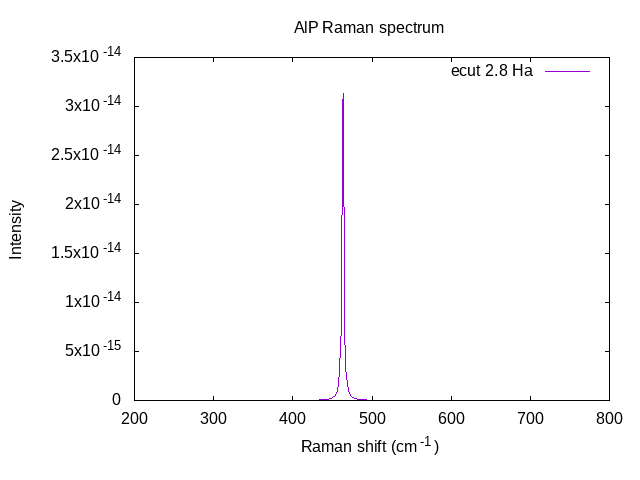
The resulting powder-average spectra, plotted here with Gnuplot, is shown below. For the cubic structure calculated here, the resulting spectra contains a single Raman TO mode corresponding to an XY polarization.
Finally, if one includes a calculation of the frequency-dependent dielectric tensor during the ANADDB calculation (see dieflag), this program extracts that dielectric tensor and prints it to its own file.