Fourth tutorial¶

Aluminum, the bulk and the surface.¶

This tutorial aims at showing how to get the following physical properties for a metal and for a surface:

the total energy
the lattice parameter
the relaxation of surface atoms
the surface energy

You will learn about the smearing of the Brillouin zone integration, and also a bit about preconditioning the SCF cycle.

This tutorial should take about 1 hour and 30 minutes.

Note

Supposing you made your own installation of ABINIT, the input files to run the examples are in the ~abinit/tests/ directory where ~abinit is the absolute path of the abinit top-level directory. If you have NOT made your own install, ask your system administrator where to find the package, especially the executable and test files.

In case you work on your own PC or workstation, to make things easier, we suggest you define some handy environment variables by executing the following lines in the terminal:

export ABI_HOME=Replace_with_absolute_path_to_abinit_top_level_dir # Change this line
export PATH=$ABI_HOME/src/98_main/:$PATH      # Do not change this line: path to executable
export ABI_TESTS=$ABI_HOME/tests/             # Do not change this line: path to tests dir
export ABI_PSPDIR=$ABI_TESTS/Pspdir/  # Do not change this line: path to pseudos dir

Examples in this tutorial use these shell variables: copy and paste the code snippets into the terminal (remember to set ABI_HOME first!) or, alternatively, source the set_abienv.sh script located in the ~abinit directory:

source ~abinit/set_abienv.sh

The ‘export PATH’ line adds the directory containing the executables to your PATH so that you can invoke the code by simply typing abinit in the terminal instead of providing the absolute path.

To execute the tutorials, create a working directory (Work*) and copy there the input files of the lesson.

Most of the tutorials do not rely on parallelism (except specific tutorials on parallelism). However you can run most of the tutorial examples in parallel with MPI, see the topic on parallelism.

Total energy and lattice parameters at fixed smearing and k-point grid¶

Before beginning, you might consider to work in a different subdirectory, as for tutorials 1, 2 or 3. Why not Work4?

The following commands will move you to your working directory, create the Work4 directory, and move you into that directory as you did in the previous tutorials. Then, we copy the file tbase4_1.abi inside the Work4 directory. The commands are:

cd $ABI_TESTS/tutorial/Input
mkdir Work4
cd Work4
cp ../tbase4_1.abi .

tbase4_1.abi is our input file. You should edit it and read it carefully,

and then a look at the following new input variables:

Note also the following:

We will work at fixed ecut (6Ha). It is implicit that in real research application, you should do a convergence test with respect to ecut. Here, a suitable ecut is given to you in order to save time. It will give a lattice parameter that is 0.2% off of the experimental value. Note that this is the softest pseudopotential of those that we have used until now: the 01h.pspgth for H needed 30 Ha (it was rather hard), the Si.psp8 for Si needed 12 Ha. See the end of this page for a discussion of soft and hard pseudopotentials.
The input variable diemac has been suppressed. Aluminum is a metal, and the default value for this input variable is tailored for that case.

When you have read the input file, you can run the code, as usual (it will take a few seconds).

abinit tbase4_1.abi > log 2> err &

Then, give a quick look at the output file. You should note that the Fermi energy and occupation numbers have been computed automatically:

Fermi (or HOMO) energy (hartree) =   0.27151   Average Vxc (hartree)=  -0.36713
Eigenvalues (hartree) for nkpt=   2  k points:
kpt#   1, nband=  3, wtk=  0.75000, kpt= -0.2500  0.5000  0.0000 (reduced coord)
  0.09836    0.25743    0.42131
    occupation numbers for kpt#   1
  2.00003    1.33305    0.00015
prteigrs : prtvol=0 or 1, do not print more k-points.

You should also note that the components of the total energy include an entropy term:

--- !EnergyTerms
iteration_state     : {dtset: 1, itime: 3, icycle: 1, }
comment             : Components of total free energy in Hartree
kinetic             :  8.68009594268178E-01
hartree             :  3.75144741427686E-03
xc                  : -1.11506134985146E+00
Ewald energy        : -2.71387012800927E+00
psp_core            :  1.56870175692757E-02
local_psp           :  1.66222476058238E-01
non_local_psp       :  4.25215770913582E-01
internal            : -2.35004517163717E+00
'-kT*entropy'       : -7.99850001032776E-03
total_energy        : -2.35804367164750E+00
total_energy_eV     : -6.41656315078440E+01
band_energy         :  3.72511439902163E-01
...

The convergence study with respect to k-points¶

There is of course a convergence study associated to the sampling of the Brillouin zone. You should examine different grids, of increasing resolution. You might try the following series of grids:

ngkpt1  2 2 2
ngkpt2  4 4 4
ngkpt3  6 6 6
ngkpt4  8 8 8

with the associated nkpt:

nkpt1  2
nkpt2 10
nkpt3 28
nkpt4 60

The input file tbase4_2.abi is an example:

while tbase4_2.abo is a reference output file:

The run might take a few seconds on a modern PC.

You will see that, for the particular value tsmear = 0.05 Ha, the lattice parameter is already converged with nkpt = 10:

acell1 7.6023827082E+00 7.6023827082E+00 7.6023827082E+00 Bohr acell2 7.5627822506E+00 7.5627822506E+00 7.5627822506E+00 Bohr acell3 7.5543007304E+00 7.5543007304E+00 7.5543007304E+00 Bohr acell4 7.5529744581E+00 7.5529744581E+00 7.5529744581E+00 Bohr

Note that there is usually a strong cross-convergence effect between the number of k-points and the value of the broadening, tsmear. The right procedure is: for each value of tsmear, convergence with respect to the number of k-points, then compare the k-point converged values for different values of tsmear.

In what follows, we will restrict ourselves to the grids with nkpt = 2, 10 and 28.

The convergence study with respect to both number of k-points and broadening factor¶

The theoretical convergence rate as a function of tsmear heading to 0, in the case of occopt = 4, is cubic. We rely on this value of occopt for this tutorial. Still, it might not be always robust, as this value might yield difficulties to find univocally the Fermi energy. A slightly worse convergence rate (quadratic) is obtained with occopt = 7, which is actually the recommended value for metallic systems.

Such convergence rates are obtained in the hypothesis of infinitely dense k-point grid. We will check the evolution of acell as a function of tsmear, for the following values of tsmear: 0.01, 0.02, 0.03 and 0.04.

Use the double-loop capability of the multi-dataset mode, with the tsmear changes in the inner loop. This will saves CPU time, as the wavefunctions of the previous dataset will be excellent (no transfer to different k-points).

The input file tbase4_3.abi is an example:

while tbase4_3.abo is the reference output file.

From the output file, here is the evolution of acell:

acell11    7.6022357792E+00  7.6022357792E+00  7.6022357792E+00 Bohr
acell12    7.6022341271E+00  7.6022341271E+00  7.6022341271E+00 Bohr
acell13    7.6022341214E+00  7.6022341214E+00  7.6022341214E+00 Bohr
acell14    7.6022357148E+00  7.6022357148E+00  7.6022357148E+00 Bohr
acell21    7.5604102145E+00  7.5604102145E+00  7.5604102145E+00 Bohr
acell22    7.5605496029E+00  7.5605496029E+00  7.5605496029E+00 Bohr
acell23    7.5565044147E+00  7.5565044147E+00  7.5565044147E+00 Bohr
acell24    7.5593333886E+00  7.5593333886E+00  7.5593333886E+00 Bohr
acell31    7.5483073963E+00  7.5483073963E+00  7.5483073963E+00 Bohr
acell32    7.5482393302E+00  7.5482393302E+00  7.5482393302E+00 Bohr
acell33    7.5497784006E+00  7.5497784006E+00  7.5497784006E+00 Bohr
acell34    7.5521340033E+00  7.5521340033E+00  7.5521340033E+00 Bohr

These data should be analyzed properly. For tsmear = 0.01, the converged value, contained in acell31, must be compared to acell11 and acell21: between acell21 and acell31, the difference is below 0.2%. acell31 can be considered to be converged with respect to the number of k-points, at fixed tsmear. This tsmear being the lowest one, it is usually the most difficult to converge, and the values acell31,32,33 and 34 are indeed well-converged with respect to the k-point number. The use of the largest tsmear = 0.04, giving acell34, induces only a small error in the lattice parameter. For that particular value of tsmear, one can use the second k-point grid, giving acell24.

Summary

So to summarize: we can choose to work with a 10 k-point grid in the irreducible Brillouin zone, and the associated tsmear = 0.04, with less than 0.1% error on the lattice parameter. Note that this error due to the Brillouin zone sampling could add to the error due to the choice of ecut (that was mentioned previously to be on the order of 0.2%).

In what follows, we will stick to these values of ecut and tsmear and try to use k-point grids with a similar resolution.

Our final value for the aluminum lattice parameter, in the LDA, using the Al.psp8 pseudopotential, is thus 7.5593 Bohr, which corresponds to 4.0002 Angstrom. The experimental value at 25 Celsius is 4.04958 Angstrom, hence our theoretical value has an error of 1.2%. We caution that converged parameters should be used to properly assess the accuracy of a pseudopotential and functional.

The associated total energy and accuracy can be deduced from:

etotal11   -2.3516656074E+00
etotal12   -2.3532597160E+00
etotal13   -2.3548538247E+00
etotal14   -2.3564479440E+00
etotal21   -2.3568282638E+00
etotal22   -2.3574128355E+00
etotal23   -2.3576771874E+00
etotal24   -2.3578584768E+00
etotal31   -2.3582092001E+00
etotal32   -2.3581800122E+00
etotal33   -2.3581917663E+00
etotal34   -2.3582884106E+00

etotal 24 is -2.3578584768E+00 Ha, with an accuracy of 0.0005 Ha.

Tip

To analyze the convergence of the total energy, one can use the abicomp.py script provide by AbiPy and the gsr command that will start an interactive ipython session so that we can interact directly with the AbiPy object. To load all the GSR files produced by calculation, use the command

abicomp.py gsr tbase4_3o*GSR.nc

then, inside the ipython terminal, execute the plot_convergence method of the GsrRobot:

In [1]: robot.plot_convergence("energy", sortby="nkpt", hue="tsmear")

to produce this plot with the total energy in eV for different values of nkpt grouped by tsmear:

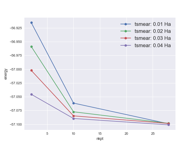
Surface energy of aluminum (100): changing the orientation of the unit cell¶

In order to study the Aluminum (100) surface, we will have to set up a supercell representing a slab. This supercell should be chosen as to be compatible with the primitive surface unit cell. The corresponding directions are [-1 1 0] and [1 1 0]. The direction perpendicular to the surface is [0 0 1]. There is no primitive cell of bulk aluminum based on these vectors, but a doubled cell. We will first compute the total energy associated with this doubled cell. This is not strictly needed, but it is a valuable intermediate step towards the study of the surface.

You might start from tbase4_3.abi. You have to change rprim. Still, try to keep acell at the values of bulk aluminum that were determined previously. But it is not all: the most difficult part in the passage to this doubled cell is the definition of the k-point grid. Of course, one could just take a homogeneous simple cubic grid of k-points, but this will not correspond exactly to the k-point grid used in the primitive cell in tbase4_3.abi. This would not be a big problem, but you would miss some error cancellation.

The answer to this problem is given in the input file $ABI_TESTS/tutorial/Input/tbase4_4.abi.

The procedure to do the exact translation of the k-point grid will not be explained here (sorry for this). If you do not see how to do it, just use homogeneous simple cubic grids, with about the same resolution as for the primitive cell case. There is a simple rule to estimate roughly whether two grids for different cells have the same resolution: simply multiply the linear dimensions of the k-point grids, by the number of sublattices, by the number of atoms in the cell. For example, the corresponding product for the usual 10 k-point grid is 4x4x4 x 4 x 1 = 256. In the file tbase4_4.in, one has 4x4x4 x 2 x 2 = 256. The grids of k-points should not be too anisotropic for this rough estimation to be valid.

Note also the input variables rprim and chkprim in this input file.

Now run tbase4_4.abi (the reference file is $ABI_TESTS/tutorial/Refs/tbase4_4.abo). You should find the following total energy:

etotal     -4.7164794308E+00

It is not exactly twice the total energy for the primitive cell, mentioned above, but the difference is less than 0.001 Ha. It is due to the different FFT grids used in the two runs, and affect the exchange-correlation energy. These grids are always homogeneous primitive 3D grids, so that changing the orientation of the lattice will give mutually incompatible lattices. Increasing the size of the FFT grid would improve the agreement.

Surface energy: a (3 aluminum layer + 1 vacuum layer) slab calculation¶

We will first compute the total energy associated with only three layers of aluminum, separated by only one layer of vacuum. This is kind of a minimal slab:

one surface layer
one “bulk” layer
one surface layer
one vacuum layer
…

It is convenient to take the vacuum region as having a multiple of the width of the aluminum layers, but this is not mandatory. The supercell to use is the double of the previous cell (that had two layers of Aluminum atoms along the [0 0 1] direction). Of course, the relaxation of the surface might give an important contribution to the total energy.

You should start from tbase4_4.abi. You have to modify rprim (double the cell along [0 0 1]), the atomic positions, as well as the k-point mesh. For the latter, it is supposed that the electrons cannot propagate from one slab to its image in the [0 0 1] direction, so that the $k_z$ component of the special k-points can be taken 0: only one layer of k-points is needed along the z-direction. You should also allow the relaxation of atomic positions, but not the relaxation of lattice parameters (the lattice parameters along x or y must be considered fixed to the bulk value, while, for the z direction, there is no interest to allow the vacuum region to collapse!

The input file tbase4_5.abi is an example,

while tbase4_5.abo is the reference output file.

The run will take a few second on a modern PC.

The total energy after the first SCF cycle, when the atomic positions are equal to their starting values, is:

ETOT  5  -7.0427135007667

The total energy of three aluminum atoms in the bulk, (from section 4.3, etotal24 multiplied by three) is -7.0735754304 Ha. Comparing the non-relaxed slab energy and the bulk energy, one obtains the non-relaxed surface energy, per surface unit cell (there are two surfaces in our simulation cell!), namely 0.01543 Ha = 0.420 eV.

The total energy after the Broyden relaxation is:

etotal     -7.0429806856E+00

The relaxed surface energy, per surface unit cell, is obtained by comparing the bulk energy and the relaxed slab energy, and gives 0.015297 Ha = 0.416 eV. It seems that the relaxation energy is very small, compared to the surface energy, but we need to do the convergence studies.

Surface energy: increasing the number of vacuum layers¶

One should now increase the number of vacuum layers: 2 and 3 layers instead of only 1. It is preferable to define atomic positions in Cartesian coordinates. The same coordinates will work for both 2 and 3 vacuum layers, while this is not the case for reduced coordinates, as the cell size increases.

The input file tbase4_6.abi is an example input file,

while tbase4_6.abo is the reference output file.

The run is on the order of of few seconds on a modern PC.

In the Broyden step 0 of the first dataset, you will notice the WARNING:

scprqt:  WARNING -
 nstep=    6 was not enough SCF cycles to converge;
 maximum force difference=  6.859E-05 exceeds toldff=  5.000E-05

The input variable nstep was intentionally set to the rather low value of 6, to warn you about possible convergence difficulties. The SCF convergence might indeed get more and more difficult with cell size. This is because the default preconditioner (see the notice of the input variable dielng) is not very good for the metal+vacuum case. For the interpretation of the present run, this is not critical, as the convergence criterion was close of being fulfilled, but one should keep this in mind, as you will see.

For the 2 vacuum layer case, one has the non-relaxed total energy:

ETOT  6  -7.0350152828531

giving the unrelaxed surface energy 0.0193 Ha = 0.525 eV; and for the relaxed case:

etotal1    -7.0358659542E+00

(this one is converged to the required level) giving the relaxed surface energy 0.0189 Ha = 0.514 eV

Note that the difference between unrelaxed and relaxed case is a bit larger than in the case of one vacuum layer. This is because there was some interaction between slabs of different supercells.

For the 3 vacuum layer case, the self-consistency is slightly more difficult than with 2 vacuum layers: the Broyden step 0 is not sufficiently converged (one might set nstep to a larger value, but the best is to change the preconditioner, as described below)… However, for the Broyden steps number 2 and beyond, because one takes advantage of the previous wavefunctions, a sufficient convergence is reached. The total energy, in the relaxed case, is:

etotal2    -7.0371360761E+00

giving the relaxed surface energy 0.0182 Ha = 0.495 eV. There is a rather small 0.019 eV difference with the 2 vacuum layer case.

For the next run, we will keep the 2 vacuum layer case, and we know that the accuracy of the coming calculation cannot be better than 0.019 eV. One might investigate the 4 vacuum layer case, but this is not worth, in the present tutorial.

Surface energy: increasing the number of aluminum layers¶

One should now increase the number of aluminum layers, while keeping 2 vacuum layers. We will consider 4 and 5 aluminum layers. This is rather straightforward to set up, but will also change the preconditioner. One could use an effective dielectric constant of about 3 or 5, with a rather small mixing coefficient, on the order of 0.2. However, there is also another possibility, using an estimation of the dielectric matrix governed by iprcel=45. For comparison with the previous treatment of SCF, one can recompute the result with 3 aluminum layers.

The input file tbase4_7.abi is an example, while

tbase4_7.abo is a reference output file.

This run might take about one minute, and is the longest of the four basic tutorials. You should start it now.

You will notice that the SCF convergence is rather satisfactory, for all the cases (3, 4 or 5 metal layers).

For the 3 aluminum layer case, one has the non-relaxed total energy:

ETOT  6  -7.0350153035193

(this quantity is converged, unlike in test 4.6) giving the unrelaxed surface energy 0.0193 Ha = 0.525 eV; and for the relaxed case:

etotal1    -7.0358683757E+00

(by contrast the difference with test 4.6 is less than 1 microHa) giving the relaxed surface energy 0.0189 Ha = 0.514 eV.

For the 4 aluminum layer case, one has the non-relaxed total energy:

ETOT  6  -9.3958299123967

giving the unrelaxed surface energy 0.0178 Ha = 0.484 eV; and for the relaxed case:

etotal2    -9.3978596458E+00

giving the relaxed surface energy 0.0168 Ha = 0.457 eV.

For the 5 aluminum layer case, one has the non-relaxed total energy:

ETOT  6  -11.754755842794

giving the unrelaxed surface energy 0.0173 Ha = 0.471 eV; and for the relaxed case:

etotal3    -1.1755343136E+01

giving the relaxed surface energy 0.0170 Ha = 0.463 eV.

The relative difference in the surface energy of the 4 and 5 layer cases is on the order of 1.2%.

In the framework of this tutorial, we will not pursue this investigation, which is a simple application of the concepts already explored.

Just for your information, and as an additional warning, when the work accomplished until now is completed with 6 and 7 layers without relaxation (see $ABI_TESTS/tutorial/Input/tbase4_8.abi and $ABI_TESTS/tutorial/Refs/tbase4_8.abo where 5, 6 and 7 layers are treated), this non-relaxed energy surface energy behaves as follows:

number of aluminum layers	surface energy
3	0.525 eV
4	0.484 eV
5	0.471 eV
6	0.419 eV
7	0.426 eV

So, the surface energy convergence is rather difficult to reach. Our values, with a 4x4x1 grid, a smearing of 0.04 Ha, a kinetic energy cut-off of 6 Ha, the Al.psp8 pseudopotential, still oscillate between 0.42 eV and 0.53 eV. Increasing the k-point sampling might decrease slightly the oscillations, but note that this effect is intrinsic to the computation of properties of a metallic surface: the electrons are confined inside the slab potential, with sub-bands in the direction normal to the surface, and the Fermi energy oscillates with the width of the slab. This effect might be understood based on a comparison with the behaviour of a jellium slab. An error on the order of 0.019 eV is due to the thin vacuum layer. Other sources of errors might have to be rechecked, seeing the kind of accuracy that is needed.

Experimental data give a surface energy around 0.55 eV (sorry, the reference is to be provided).

Soft and hard pseudopotentials¶

In the context of a plane-wave basis, a soft pseudopotential means that a low ecut will be required to obtain convergence whereas a hard pseudopotential implies that a high ecut will be needed. It can be understood by considering the pseudo-wave-functions of that atom. A hard pseudopotential has pseudo-wave-functions that have sharp features in real space which require many plane-waves to describe.

On the other hand, a soft pseudopotential has rather smooth pseudo-wave-functions that need fewer plane-waves to describe accurately than the pseudo-wave-functions of hard pseudopotentials. This designation is somewhat qualitative, and it is relative to other pseudopotentials. In other words, a pseudopotential can be soft when compared to a certain pseudopotential but hard with respect to another.

In general, pseudopotentials describing light elements, those of the 2^nd line of the periodic table, and pseudopotentials that include semi-core states are considered hard as they have strongly peaked pseudo-wave-functions that require a large ecut. This discussion is valid for norm-conserving pseudopotentials. With PAW pseudopotentials, we are able to keep pseudo-wave-function smooth which means that they will require lower ecut than their norm-conserving counterpart which is one of their main benefits.