First tutorial on GWR (GW in real-space and imaginary time)
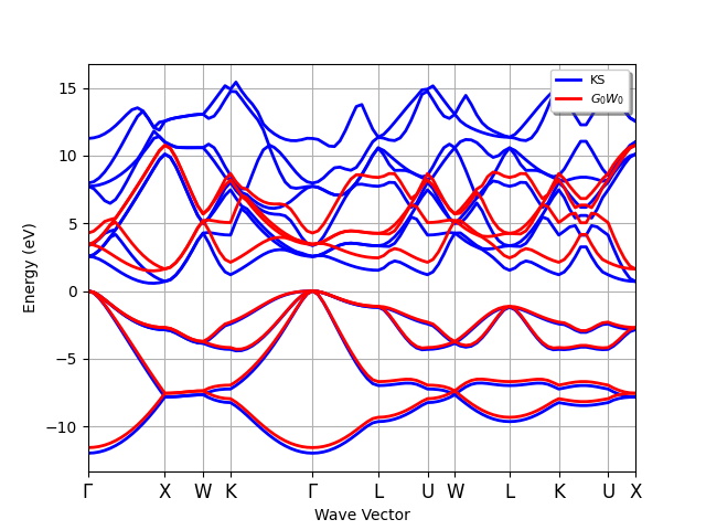
The quasi-particle band structure of Silicon in the one-shot GW approximation.
This tutorial aims at showing how to calculate self-energy corrections to the DFT Kohn-Sham (KS) eigenvalues in the one-shot GW approximation using the GWR code
The user should be already familiar with the four basic tutorials of ABINIT, see the tutorial home page, and is strongly encouraged to read the introduction to the GWR code before running these examples.
This tutorial should take about 1.5 hours.
Note
Supposing you made your own installation of ABINIT, the input files to run the examples are in the ~abinit/tests/ directory where ~abinit is the absolute path of the abinit top-level directory. If you have NOT made your own install, ask your system administrator where to find the package, especially the executable and test files.
In case you work on your own PC or workstation, to make things easier, we suggest you define some handy environment variables by executing the following lines in the terminal:
export ABI_HOME=Replace_with_absolute_path_to_abinit_top_level_dir # Change this line
export PATH=$ABI_HOME/src/98_main/:$PATH      # Do not change this line: path to executable
export ABI_TESTS=$ABI_HOME/tests/             # Do not change this line: path to tests dir
export ABI_PSPDIR=$ABI_TESTS/Pspdir/  # Do not change this line: path to pseudos dir
Examples in this tutorial use these shell variables: copy and paste
the code snippets into the terminal (remember to set ABI_HOME first!) or, alternatively,
source the set_abienv.sh script located in the ~abinit directory:
source ~abinit/set_abienv.sh
The ‘export PATH’ line adds the directory containing the executables to your PATH so that you can invoke the code by simply typing abinit in the terminal instead of providing the absolute path.
To execute the tutorials, create a working directory (Work*) and
copy there the input files of the lesson.
Most of the tutorials do not rely on parallelism (except specific tutorials on parallelism). However you can run most of the tutorial examples in parallel with MPI, see the topic on parallelism.
Ground-state and KS band structure
Before beginning, you might consider creating a different subdirectory to work in. Why not create Work_gwr?
The file tgwr_1.abi is the input file for the first step: a SCF run followed by a KS NSCF band structure calculation along a high-symmetry \(\kk\)-path. Copy it to the working directory with:
mkdir Work_gwr
cd Work_gwr
cp ../tgwr_1.abi .
You may want to immediately start the job in background with:
mpirun -n 1 tgwr_1.abi > tgwr_1.log 2> err &
so that we have some time to discuss the input while ABINIT is running.
# Crystalline silicon. Preparatory run for GWR code
# Dataset 1: ground state calculation to compute the density.
# Dataset 2: KS band structure calculation along a k-path.

# Include geometry and pseudos
include "gwr_include.abi"

ndtset 2
prtwf -1       # Don't need wavefunctions.

#paral_kgb 1   # Activate spin/k-point/band/FFT
#autoparal 1   # Automatic selection of np* variables.
#npfft 1       # Disable MPI-FFT

####################
# Dataset 1: SCF run
####################
nband1  6

# Definition of the k-point grid
ngkpt1   4 4 4
nshiftk1 4
shiftk1  0.0 0.0 0.0
         0.0 0.5 0.5
         0.5 0.0 0.5
         0.5 0.5 0.0
tolvrs1 1.e-12

#######################################
# Dataset 2: Band structure calculation
#######################################
getden2    -1
nband2      12
nbdbuf2     4
tolwfr2     1e-20
iscf2      -2   # NSCF run

# K-path in reduced coordinates:
# Generate using `abistruct.py kpath gwr_include.abi`
ndivsm2 5
kptopt2 -11
kptbounds2
   +0.000000000  +0.000000000  +0.000000000  # $\Gamma$
   +0.500000000  +0.000000000  +0.500000000  # X
   +0.500000000  +0.250000000  +0.750000000  # W
   +0.375000000  +0.375000000  +0.750000000  # K
   +0.000000000  +0.000000000  +0.000000000  # $\Gamma$
   +0.500000000  +0.500000000  +0.500000000  # L
   +0.625000000  +0.250000000  +0.625000000  # U
   +0.500000000  +0.250000000  +0.750000000  # W
   +0.500000000  +0.500000000  +0.500000000  # L
   +0.375000000  +0.375000000  +0.750000000  # K
   +0.625000000  +0.250000000  +0.625000000  # U
   +0.500000000  +0.000000000  +0.500000000  # X


# Definition of the SCF procedure
nstep   100       # Maximal number of SCF cycles
diemac  12.0      # Although this is not mandatory, it is worth to
                  # precondition the SCF cycle. The model dielectric
                  # function used as the standard preconditioner
                  # is described in the "dielng" input variable section.
                  # Here, we follow the prescription for bulk silicon.

#%%<BEGIN TEST_INFO>
#%% [setup]
#%% executable = abinit
#%% test_chain = tgwr_1.abi, tgwr_2.abi, tgwr_3.abi, tgwr_4.abi, tgwr_5.abi
#%% need_cpp_vars = HAVE_LINALG_SCALAPACK
#%% exclude_builders = eos_nvhpc_23.9_elpa ,eos_nvhpc_24.9_openmpi, haicgu_*
#%% [shell]
#%% pre_commands = iw_cp gwr_include.abi gwr_include.abi
#%% [files]
#%% files_to_test =
#%%   tgwr_1.abo, tolnlines = 25, tolabs = 1.1e-3, tolrel = 3.0e-3, fld_options = -medium;
#%% [paral_info]
#%% max_nprocs = 12
#%% [extra_info]
#%% authors = M. Giantomassi
#%% keywords = NC, GWR
#%% description =
#%%     Crystalline silicon. Preparatory run for GWR code
#%%     Dataset 1: ground state calculation to compute the density.
#%%     Dataset 2: KS band structure calculation along a k-path.
#%%<END TEST_INFO>
Tip
All the input files of this tutorial can be executed in parallel by just
increasing the value of NUM in mpirun -n NUM.
Clearly the size of the problem is small so do not expect
great parallel performance if you start to use dozens of MPI processes.
The first dataset produces the KS density file that is then used to compute the band structure in the second dataset. Since all the input files of this tutorial use the same crystalline structure, pseudos and cutoff energy ecut for the wavefunctions, we declare these variables in an external file that will be included in all the other input files using the syntax:
# Include geometry and pseudos
include "gwr_include.abi"
If you open the include file:
ecut 16.0        # Maximal kinetic energy cut-off, in Hartree

# Definition of the unit cell: fcc
acell  3*10.26         # Experimental lattice constants in Bohr
rprim  0.0  0.5  0.5   # FCC primitive vectors (to be scaled by acell)
       0.5  0.0  0.5
       0.5  0.5  0.0

# Definition of the atom types
ntypat  1
znucl 14

# Definition of the atoms
natom  2
typat  1 1
xred
      0.0  0.0  0.0
      0.25 0.25 0.25

# PBE pseudos from the PseudoDojo (scalar relativistic)
pp_dirpath "$ABI_PSPDIR"
pseudos "Psdj_nc_sr_04_pbe_std_psp8/Si.psp8"
you will notice that we are using norm-conserving (NC) pseudos taken from the standard scalar-relativistic table of the PseudoDojo, and the recommended value for ecut reported in the PseudoDojo table (16 Ha, normal hint).
Important
For GW calculations, we strongly recommend using NC pseudos from the stringent table as these pseudos have closed-shells treated as valence states. This is important for a correct description of the matrix elements of the exchange part of the self-energy that are rather sensitive to the overlap between the wavefunctions [Setten2018]. In the special case of silicon, there is no difference between the standard version and the stringent version of the pseudo, but if we consider e.g. Ga, you will notice that the stringent version includes all the 3spd states in valence besides the outermost 4sp electrons whereas the standard pseudo for Ga designed for GS calculations includes only the 3d states.
At this point, the calculation should have completed, and we can have a look at the KS band structure to find the position of the band edges.
Tip
If AbiPy is installed on your machine, you can use the abiopen.py script
with the --expose option to visualize the band structure from the GSR.nc file:
abiopen.py tgwr_1o_DS2_GSR.nc --expose
To print the results to terminal, use:
abiopen.py tgwr_1o_DS2_GSR.nc -p
============================== Electronic Bands ==============================
Number of electrons: 8.0, Fermi level: 4.356 (eV)
nsppol: 1, nkpt: 101, mband: 12, nspinor: 1, nspden: 1
smearing scheme: none (occopt 1), tsmear_eV: 0.272, tsmear Kelvin: 3157.7
Direct gap:
    Energy: 2.556 (eV)
    Initial state: spin: 0, kpt: $\Gamma$ [+0.000, +0.000, +0.000], band: 3, eig: 4.356, occ: 2.000
    Final state:   spin: 0, kpt: $\Gamma$ [+0.000, +0.000, +0.000], band: 4, eig: 6.912, occ: 0.000
Fundamental gap:
    Energy: 0.570 (eV)
    Initial state: spin: 0, kpt: $\Gamma$ [+0.000, +0.000, +0.000], band: 3, eig: 4.356, occ: 2.000
    Final state:   spin: 0, kpt: [+0.429, +0.000, +0.429], band: 4, eig: 4.926, occ: 0.000
Bandwidth: 11.970 (eV)
Valence maximum located at kpt index 0:
    spin: 0, kpt: $\Gamma$ [+0.000, +0.000, +0.000], band: 3, eig: 4.356, occ: 2.000
Conduction minimum located at kpt index 12:
    spin: 0, kpt: [+0.429, +0.000, +0.429], band: 4, eig: 4.926, occ: 0.000
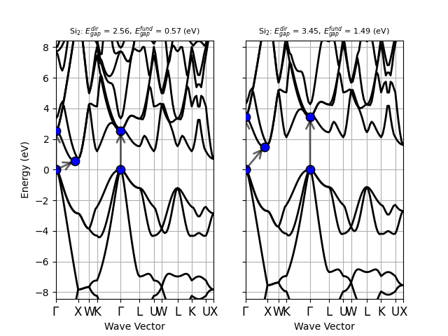
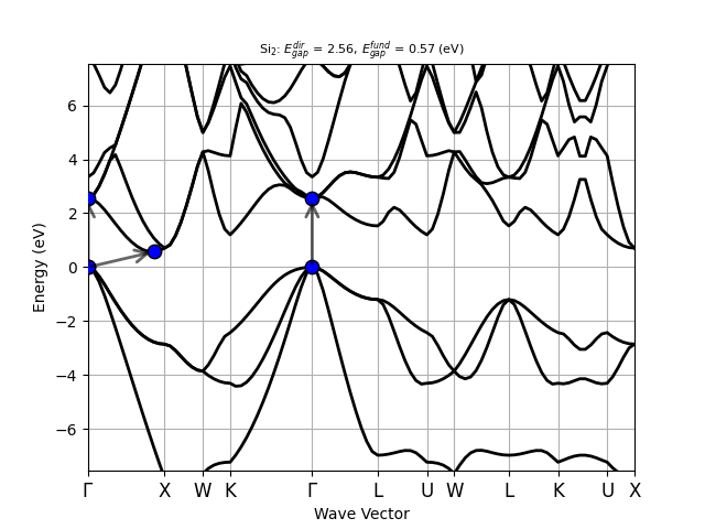
Silicon is an indirect band gap semiconductor: the CBM is located at the \(\Gamma\) point while the VMB is located at ~[+0.429, +0.000, +0.429]. At the PBE level, the direct gap is 2.556 eV while the fundamental band gap is ~0.570 eV. Both values strongly underestimate the experimental results that are ~3.4 eV and ~1.12 eV, respectively.
Important
Similarly to the conventional GW code, also the GWR code can compute QP corrections only for the \(\kk\)-points belonging to the \(\kk\)-mesh associated to the WFK file. Before running GW calculations is always a good idea to analyze carefully the KS band structure in order to understand the location of the band edges and then select the most appropriate \(\kk\)-mesh.
One final comment related to the MPI parallelism in the ground-state part. For larger system, it is advisable to use paral_kgb = 1 for its better scalability in conjunction with autoparal 1 to allow ABINIT to determine an optimal distribution, in particular the band parallelism that is not available when the CG eigensolver is used.
Generation of the WFK file with empty states
In the second input file, we use the density file computed previously (tgwr_1o_DS1_DEN)
to generate WFK files with three different \(\Gamma\)-centered \(\kk\)-meshes:
ndtset 3

ngkpt1   2 2 2
ngkpt2   4 4 4
ngkpt3   6 6 6
This allows us to perform convergence studies with respect to the BZ sampling. Let us recall that shifted \(\kk\)-meshes are not supported by GWR. In another words, nshiftk must be set to 1 with shiftk = 0 0 0 when producing the WFK file. The density file, on the contrary, can be generated with shifted \(\kk\)-meshes, as usual.
Let’s immediately start the job in background with:
mpirun -n 1 tgwr_2.abi > tgwr_2.log 2> err &
#  Calculation of WFK files with empty states and direct diagonalization

# Include geometry and pseudos
include "gwr_include.abi"

# Generate 3 WFK files with increased BZ sampling.
ndtset 3
ngkpt1 2 2 2
ngkpt2 4 4 4
ngkpt3 6 6 6

# Definition of the k-point grid
# IMPORTANT: GWR requires Gamma-centered k-meshes
nshiftk 1
shiftk  0.0 0.0 0.0

###########################################
# Direct diago with empty states
###########################################
optdriver  6                         # Activate GWR code
gwr_task "HDIAGO"                    # Direct diagonalization
nband     400                        # Number of (occ + empty) bands
getden_filepath "tgwr_1o_DS1_DEN"    # Density file used to build H[n]

#%%<BEGIN TEST_INFO>
#%% [setup]
#%% executable = abinit
#%% test_chain = tgwr_1.abi, tgwr_2.abi, tgwr_3.abi, tgwr_4.abi, tgwr_5.abi
#%% need_cpp_vars = HAVE_LINALG_SCALAPACK
#%% exclude_builders = eos_nvhpc_23.9_elpa ,eos_nvhpc_24.9_openmpi, haicgu_*
#%% [files]
#%% files_to_test =
#%%   tgwr_2.abo, tolnlines = 25, tolabs = 1.1e-3, tolrel = 3.0e-3, fld_options = -medium;
#%% [paral_info]
#%% max_nprocs = 12
#%% [extra_info]
#%% authors = M. Giantomassi
#%% keywords = NC, GWR
#%% description =
#%%  Calculation of WFK files with empty states with direct diagonalization
#%%<END TEST_INFO>
Here we are using gwr_task = “HDIAGO” to perform a direct diagonalization of the KS Hamiltonian \(H^\KS[n]\) constructed from the input DEN file. This procedure differs from the one used in the other GW tutorials in which the WFK file is generated by performing an iterative diagonalization in which only the application of the Hamiltonian is required. The reason is that the direct diagonalization outperforms iterative methods when many empty states are required, especially if one can take advantage of ScalaPack to distribute the KS Hamiltonian matrix.
Important
We strongly recommend using the ELPA library for diagonalization, as it is much more efficient and requires significantly less memory than the ScaLAPACK drivers. See the GWR_intro for more details on how to link the ELPA library.
Here, we ask for 400 bands. Let’s recall that in the previous GW tutorial nband = 100 was considered converged within 30 meV, but with GWR we can afford more bands since nband enters into play only during the initial construction of the Green’s function Clearly, when studying new systems, the value of nband needed to converge is not known beforehand. Therefore, it is important to plan ahead and choose a reasonably large number of bands to avoid regenerating the WFK file multiple times just to increase nband.
Note also that paral_kgb = 1 is only available in the ground-state (GS) part. The GWR code, indeed, employs its own distribution scheme, which depends on the value of gwr_task. When “HDIAGO” is used, the distribution is handled automatically at runtime, and the user has no control over it. Please refer to the note below for guidance on choosing an appropriate number of MPI processes to ensure an efficient workload distribution.
Important
The direct diagonalization is MPI-parallelized across three different levels: collinear spin \(\sigma\) (not used here), \(\kk\)-points in the IBZ and Scalapack distribution of the \(H^\sigma_\kk(\bg,\bg')\) matrix. ABINIT will try to find an “optimal” distribution of the workload at runtime, yet there are a couple of things worth keeping in mind when choosing the number of MPI processes for this step. Ideally the total number of cores should be a multiple of nkpt * nsppol to avoid load imbalance.
In order to compute all the eigenvectors of the KS Hamiltonian, one can use gwr_task “HDIAGO_FULL”. In this case the value of nband is automatically set to the total number of plawewaves for that particular \(\kk\)-point. No stopping criterion such as tolwfr or number of iterations nstep are required when Scalapack is used.
Again, multi-datasets are strongly discouraged if you care about performance.
Our first GWR calculation
For our first GWR run, we use a minimalistic input file that performs a GWR calculation using the DEN and the WFK file produced previously. First of all, you may want to start immediately the computation with:
mpirun -n 1 tgwr_3.abi > tgwr_3.log 2> err &
and the following input file:
# Crystalline silicon
# Calculation of one-shot GW corrections with GWR code.

# Definition of the k-point grid
# IMPORTANT: GWR requires Gamma-centered k-meshes
ngkpt   2 2 2
nshiftk 1
shiftk  0.0 0.0 0.0

# Include geometry and pseudos
include "gwr_include.abi"

################################
# Dataset 3: G0W0 with GWR code
################################
optdriver  6                          # Activate GWR code
ecutwfn    10                         # Truncate basis set when computing G.
                                      # This parameter should be subject to convergence studies
gwr_task "G0W0"                       # One-shot calculation
getden_filepath "tgwr_1o_DS1_DEN"     # Density file
getwfk_filepath "tgwr_2o_DS1_WFK"     # WFK file with empty states and 2x2x2 k-mesh

gwr_ntau 6          # Number of minimax points
gwr_boxcutmin  1.0  # This should be subject to convergence studies
gwr_sigma_algo 2    # Use convolutions in the BZ for Sigma

nband      100      # Bands to be used in Green's functions.
ecuteps    6        # Cut-off energy of the planewave set to represent the dielectric matrix.
                    # It is important to adjust this parameter.
#ecutsigx    16     # Dimension of the G sum in Sigma_x.

nkptgw      2       # number of k-point where to calculate the GW correction
kptgw               # k-points in reduced coordinates
   0.0    0.0    0.0
   0.5    0.0    0.0

bdgw       # calculate GW corrections for bands from 4 to 5
   4  5
   4  5

# Spectral function (very coarse grid to reduce txt file size)
#nfreqsp3 50
#freqspmax3 5 eV

#%%<BEGIN TEST_INFO>
#%% [setup]
#%% executable = abinit
#%% test_chain = tgwr_1.abi, tgwr_2.abi, tgwr_3.abi, tgwr_4.abi, tgwr_5.abi
#%% need_cpp_vars = HAVE_LINALG_SCALAPACK
#%% exclude_builders = eos_nvhpc_23.9_elpa ,eos_nvhpc_24.9_openmpi, haicgu_*
#%% [files]
#%% files_to_test =
#%%   tgwr_3.abo, tolnlines = 50, tolabs = 1.1e-3, tolrel = 3.0e-3, fld_options = -medium;
#%% [paral_info]
#%% max_nprocs = 12
#%% [extra_info]
#%% authors = M. Giantomassi
#%% keywords = NC, GWR
#%% description =
#%%  Crystalline silicon
#%%  Calculation of one-shot GW corrections with GWR code.
#%%<END TEST_INFO>
This input contains some variables whose meaning is the same as in the conventional GW code,
and other variables whose name starts with gwr_ that are specific to the GWR code.
We use optdriver 6 to enter the GWR code while gwr_task activates a one-shot GW calculation. To reduce the wall-time, we use a minimax mesh with gwr_ntau = 6 points, the minimum number of points that can be used. Most likely, six points are not sufficient, but the convergence study for gwr_ntau is postponed to the next sections. getden_filepath specifies the density file used to compute \(v_{xc}[n](\rr)\), while getwfk_filepath specifies the WFK file with empty states used to build the Green’s function.
Important
Keep in mind that the \(\kk\)-mesh specified in the input via ngkpt, nshiftk and shiftk must agree with the one found in the WFK file else the code will abort.
Also, the FFT mesh for the density ngfft specified in the input must agree with the one found in the DEN.
This is usually true, provided that the same ecut value is used everywhere.
A possible exception occurs when using paral_kgb 1 with MPI-FFT (npfft > 1) to generate the DEN.
In this case, the last two dimensions of the FFT mesh must be multiples of npfft.
Since MPI-FFT is not available in GWR, ABINIT will stop with an error, complaining that the ngfft mesh
computed from the input does not match the one read from the file.
To solve the problem, simply set ngfft explicitly in the GWR input files using the value used in the GS part.
To accelerate the computation and reduce the memory requirements, we truncate the PW basis set using ecutwfn = 10 < ecut = 16, and gwr_boxcutmin is set to 1.0. These parameters should be subject to carefully convergence studies as systems with localized electrons such as 3d or 4f electrons may require larger values (more PWs and denser FFT meshes). Please take some time to read the variable description of ecutwfn and gwr_boxcutmin before proceeding.
Now, let us turn our attention to the variables that are also used in the conventional GW code. The cutoff of the polarizability and \(W\) is defined by ecuteps as in the conventional GW code. The cutoff for the exchange part of the self-energy is given by ecutsigx. For the initial convergence studies, it is advised to set ecutsigx to a value as high as ecut since, anyway, this parameter is not much influential on the total computational time, as only occupied states are involved. Note that the exact treatment of the exchange part requires, in principle, ecutsigx = 4 * ecut.
The \(\kk\)-points and the band range for the QP corrections are set expliclty via nkptgw, kptgw and bdgw.
We can now have a look at the main output file:
.Version 10.5.8.2 of ABINIT, released Oct 2025.
.(MPI version, prepared for a x86_64_linux_gnu13.2 computer)
.Copyright (C) 1998-2026 ABINIT group .
ABINIT comes with ABSOLUTELY NO WARRANTY.
It is free software, and you are welcome to redistribute it
under certain conditions (GNU General Public License,
see ~abinit/COPYING or http://www.gnu.org/copyleft/gpl.txt).
ABINIT is a project of the Universite Catholique de Louvain,
Corning Inc. and other collaborators, see ~abinit/doc/developers/contributors.txt .
Please read https://docs.abinit.org/theory/acknowledgments for suggested
acknowledgments of the ABINIT effort.
For more information, see https://www.abinit.org .
.Starting date : Sat 20 Dec 2025.
- ( at 17h07 )
- input file -> /home/buildbot/ABINIT3/eos_gnu_13.2_mpich/trunk__codata2022/tests/TestBot_MPI1/tutorial_tgwr_1-tgwr_2-tgwr_3-tgwr_4-tgwr_5/tgwr_3.abi
- output file -> tgwr_3.abo
- root for input files -> tgwr_3i
- root for output files -> tgwr_3o
Symmetries : space group Fd -3 m (#227); Bravais cF (face-center cubic)
================================================================================
Values of the parameters that define the memory need of the present run
intxc = 0 ionmov = 0 iscf = 7 lmnmax = 6
lnmax = 6 mgfft = 30 mpssoang = 3 mqgrid = 3001
natom = 2 nloc_mem = 1 nspden = 1 nspinor = 1
nsppol = 1 nsym = 48 n1xccc = 2501 ntypat = 1
occopt = 1 xclevel = 2
- mband = 100 mffmem = 1 mkmem = 3
mpw = 435 nfft = 27000 nkpt = 3
================================================================================
P This job should need less than 11.418 Mbytes of memory.
Rough estimation (10% accuracy) of disk space for files :
_ WF disk file : 1.993 Mbytes ; DEN or POT disk file : 0.208 Mbytes.
================================================================================
--------------------------------------------------------------------------------
------------- Echo of variables that govern the present computation ------------
--------------------------------------------------------------------------------
-
- outvars: echo of selected default values
- iomode0 = 0 , fftalg0 =512 , wfoptalg0 = 0
-
- outvars: echo of global parameters not present in the input file
- max_nthreads = 0
-
-outvars: echo values of preprocessed input variables --------
acell 1.0260000000E+01 1.0260000000E+01 1.0260000000E+01 Bohr
amu 2.80855000E+01
bdgw 4 5 4 5
ecut 1.60000000E+01 Hartree
ecuteps 6.00000000E+00 Hartree
ecutsigx 1.60000000E+01 Hartree
ecutwfn 1.00000000E+01 Hartree
- fftalg 512
gwr_ntau 6
gwr_sigma_algo 2
istwfk 2 3 7
ixc 11
kpt 0.00000000E+00 0.00000000E+00 0.00000000E+00
5.00000000E-01 0.00000000E+00 0.00000000E+00
5.00000000E-01 5.00000000E-01 0.00000000E+00
kptgw 0.00000000E+00 0.00000000E+00 0.00000000E+00
5.00000000E-01 0.00000000E+00 0.00000000E+00
kptrlatt 2 0 0 0 2 0 0 0 2
kptrlen 1.45098311E+01
P mkmem 3
natom 2
nband 100
ngfft 30 30 30
nkpt 3
nkptgw 2
nsym 48
ntypat 1
occ 2.000000 2.000000 2.000000 2.000000 0.000000 0.000000
0.000000 0.000000 0.000000 0.000000 0.000000 0.000000
0.000000 0.000000 0.000000 0.000000 0.000000 0.000000
0.000000 0.000000 0.000000 0.000000 0.000000 0.000000
0.000000 0.000000 0.000000 0.000000 0.000000 0.000000
0.000000 0.000000 0.000000 0.000000 0.000000 0.000000
0.000000 0.000000 0.000000 0.000000 0.000000 0.000000
0.000000 0.000000 0.000000 0.000000 0.000000 0.000000
0.000000 0.000000 0.000000 0.000000 0.000000 0.000000
0.000000 0.000000 0.000000 0.000000 0.000000 0.000000
0.000000 0.000000 0.000000 0.000000 0.000000 0.000000
0.000000 0.000000 0.000000 0.000000 0.000000 0.000000
0.000000 0.000000 0.000000 0.000000 0.000000 0.000000
0.000000 0.000000 0.000000 0.000000 0.000000 0.000000
0.000000 0.000000 0.000000 0.000000 0.000000 0.000000
0.000000 0.000000 0.000000 0.000000 0.000000 0.000000
0.000000 0.000000 0.000000 0.000000
optdriver 6
rprim 0.0000000000E+00 5.0000000000E-01 5.0000000000E-01
5.0000000000E-01 0.0000000000E+00 5.0000000000E-01
5.0000000000E-01 5.0000000000E-01 0.0000000000E+00
spgroup 227
symrel 1 0 0 0 1 0 0 0 1 -1 0 0 0 -1 0 0 0 -1
0 -1 1 0 -1 0 1 -1 0 0 1 -1 0 1 0 -1 1 0
-1 0 0 -1 0 1 -1 1 0 1 0 0 1 0 -1 1 -1 0
0 1 -1 1 0 -1 0 0 -1 0 -1 1 -1 0 1 0 0 1
-1 0 0 -1 1 0 -1 0 1 1 0 0 1 -1 0 1 0 -1
0 -1 1 1 -1 0 0 -1 0 0 1 -1 -1 1 0 0 1 0
1 0 0 0 0 1 0 1 0 -1 0 0 0 0 -1 0 -1 0
0 1 -1 0 0 -1 1 0 -1 0 -1 1 0 0 1 -1 0 1
-1 0 1 -1 1 0 -1 0 0 1 0 -1 1 -1 0 1 0 0
0 -1 0 1 -1 0 0 -1 1 0 1 0 -1 1 0 0 1 -1
1 0 -1 0 0 -1 0 1 -1 -1 0 1 0 0 1 0 -1 1
0 1 0 0 0 1 1 0 0 0 -1 0 0 0 -1 -1 0 0
1 0 -1 0 1 -1 0 0 -1 -1 0 1 0 -1 1 0 0 1
0 -1 0 0 -1 1 1 -1 0 0 1 0 0 1 -1 -1 1 0
-1 0 1 -1 0 0 -1 1 0 1 0 -1 1 0 0 1 -1 0
0 1 0 1 0 0 0 0 1 0 -1 0 -1 0 0 0 0 -1
0 0 -1 0 1 -1 1 0 -1 0 0 1 0 -1 1 -1 0 1
1 -1 0 0 -1 1 0 -1 0 -1 1 0 0 1 -1 0 1 0
0 0 1 1 0 0 0 1 0 0 0 -1 -1 0 0 0 -1 0
-1 1 0 -1 0 0 -1 0 1 1 -1 0 1 0 0 1 0 -1
0 0 1 0 1 0 1 0 0 0 0 -1 0 -1 0 -1 0 0
1 -1 0 0 -1 0 0 -1 1 -1 1 0 0 1 0 0 1 -1
0 0 -1 1 0 -1 0 1 -1 0 0 1 -1 0 1 0 -1 1
-1 1 0 -1 0 1 -1 0 0 1 -1 0 1 0 -1 1 0 0
tnons 0.0000000 0.0000000 0.0000000 0.2500000 0.2500000 0.2500000
0.0000000 0.0000000 0.0000000 0.2500000 0.2500000 0.2500000
0.0000000 0.0000000 0.0000000 0.2500000 0.2500000 0.2500000
0.0000000 0.0000000 0.0000000 0.2500000 0.2500000 0.2500000
0.0000000 0.0000000 0.0000000 0.2500000 0.2500000 0.2500000
0.0000000 0.0000000 0.0000000 0.2500000 0.2500000 0.2500000
0.0000000 0.0000000 0.0000000 0.2500000 0.2500000 0.2500000
0.0000000 0.0000000 0.0000000 0.2500000 0.2500000 0.2500000
0.0000000 0.0000000 0.0000000 0.2500000 0.2500000 0.2500000
0.0000000 0.0000000 0.0000000 0.2500000 0.2500000 0.2500000
0.0000000 0.0000000 0.0000000 0.2500000 0.2500000 0.2500000
0.0000000 0.0000000 0.0000000 0.2500000 0.2500000 0.2500000
0.0000000 0.0000000 0.0000000 0.2500000 0.2500000 0.2500000
0.0000000 0.0000000 0.0000000 0.2500000 0.2500000 0.2500000
0.0000000 0.0000000 0.0000000 0.2500000 0.2500000 0.2500000
0.0000000 0.0000000 0.0000000 0.2500000 0.2500000 0.2500000
0.0000000 0.0000000 0.0000000 0.2500000 0.2500000 0.2500000
0.0000000 0.0000000 0.0000000 0.2500000 0.2500000 0.2500000
0.0000000 0.0000000 0.0000000 0.2500000 0.2500000 0.2500000
0.0000000 0.0000000 0.0000000 0.2500000 0.2500000 0.2500000
0.0000000 0.0000000 0.0000000 0.2500000 0.2500000 0.2500000
0.0000000 0.0000000 0.0000000 0.2500000 0.2500000 0.2500000
0.0000000 0.0000000 0.0000000 0.2500000 0.2500000 0.2500000
0.0000000 0.0000000 0.0000000 0.2500000 0.2500000 0.2500000
typat 1 1
wtk 0.12500 0.50000 0.37500
xangst 0.0000000000E+00 0.0000000000E+00 0.0000000000E+00
1.3573395450E+00 1.3573395450E+00 1.3573395450E+00
xcart 0.0000000000E+00 0.0000000000E+00 0.0000000000E+00
2.5650000000E+00 2.5650000000E+00 2.5650000000E+00
xred 0.0000000000E+00 0.0000000000E+00 0.0000000000E+00
2.5000000000E-01 2.5000000000E-01 2.5000000000E-01
znucl 14.00000
================================================================================
chkinp: Checking input parameters for consistency.
================================================================================
== DATASET 1 ==================================================================
- mpi_nproc: 1, omp_nthreads: -1 (-1 if OMP is not activated)
--- !DatasetInfo
iteration_state: {dtset: 1, }
dimensions: {natom: 2, nkpt: 3, mband: 100, nsppol: 1, nspinor: 1, nspden: 1, mpw: 435, }
cutoff_energies: {ecut: 16.0, pawecutdg: -1.0, }
electrons: {nelect: 8.00000000E+00, charge: 0.00000000E+00, occopt: 1.00000000E+00, tsmear: 1.00000000E-02, }
meta: {optdriver: 6, }
...
mkfilename: getwfk from: tgwr_2o_DS1_WFK
mkfilename: getden from: tgwr_1o_DS1_DEN
Exchange-correlation functional for the present dataset will be:
GGA: Perdew-Burke-Ernzerhof functional - ixc=11
Citation for XC functional:
J.P.Perdew, K.Burke, M.Ernzerhof, PRL 77, 3865 (1996)
.Using double precision arithmetic; gwpc = 8
- Reading GS density from: tgwr_1o_DS1_DEN
--- Pseudopotential description ------------------------------------------------
- pspini: atom type 1 psp file is /home/buildbot/ABINIT3/eos_gnu_13.2_mpich/trunk__codata2022/tests/Pspdir/Psdj_nc_sr_04_pbe_std_psp8/Si.psp8
- pspatm: opening atomic psp file /home/buildbot/ABINIT3/eos_gnu_13.2_mpich/trunk__codata2022/tests/Pspdir/Psdj_nc_sr_04_pbe_std_psp8/Si.psp8
- Si ONCVPSP-3.2.3.1 r_core= 1.60303 1.72197 1.91712
- 14.00000 4.00000 170510 znucl, zion, pspdat
8 11 2 4 600 0.00000 pspcod,pspxc,lmax,lloc,mmax,r2well
5.99000000000000 4.00000000000000 0.00000000000000 rchrg,fchrg,qchrg
nproj 2 2 2
extension_switch 1
pspatm : epsatm= 9.34321699
--- l ekb(1:nproj) -->
0 5.168965 0.829883
1 2.571282 0.578307
2 -2.427311 -0.488097
pspatm: atomic psp has been read and splines computed
1.49491472E+02 ecore*ucvol(ha*bohr**3)
--------------------------------------------------------------------------------
Total charge density [el/Bohr^3]
) Maximum= 8.5569E-02 at reduced coord. 0.1000 0.1000 0.7000
) Minimum= 1.4870E-03 at reduced coord. 0.0000 0.0000 0.0000
Integrated= 8.0000E+00
- Reading GS states from WFK file: tgwr_2o_DS1_WFK
Mapping kBZ --> kIBZ
Legend: bz = TS(ibz) + g0 where isym is the index of the symrec operation S and itim is 1 if TR is used.
BZ IBZ ibz isym itim g0
1 [ 0.0000E+00, 0.0000E+00, 0.0000E+00] [ 0.0000E+00, 0.0000E+00, 0.0000E+00] 1 1 0 [0, 0, 0]
2 [ 5.0000E-01, 0.0000E+00, 0.0000E+00] [ 5.0000E-01, 0.0000E+00, 0.0000E+00] 2 1 0 [0, 0, 0]
3 [ 5.0000E-01, 5.0000E-01, 5.0000E-01] [ 5.0000E-01, 0.0000E+00, 0.0000E+00] 2 5 0 [1, 1, 1]
4 [ 0.0000E+00, 0.0000E+00, 5.0000E-01] [ 5.0000E-01, 0.0000E+00, 0.0000E+00] 2 3 0 [0, 0, 0]
5 [ 0.0000E+00, 5.0000E-01, 0.0000E+00] [ 5.0000E-01, 0.0000E+00, 0.0000E+00] 2 7 0 [0, 0, 0]
6 [ 5.0000E-01, 5.0000E-01, 0.0000E+00] [ 5.0000E-01, 5.0000E-01, 0.0000E+00] 3 1 0 [0, 0, 0]
7 [ 5.0000E-01, 0.0000E+00, 5.0000E-01] [ 5.0000E-01, 5.0000E-01, 0.0000E+00] 3 9 0 [1, 0, 1]
8 [ 0.0000E+00, 5.0000E-01, 5.0000E-01] [ 5.0000E-01, 5.0000E-01, 0.0000E+00] 3 17 0 [0, 0, 0]
Mapping qBZ --> qIBZ
Legend: bz = TS(ibz) + g0 where isym is the index of the symrec operation S and itim is 1 if TR is used.
BZ IBZ ibz isym itim g0
1 [ 0.0000E+00, 0.0000E+00, 0.0000E+00] [ 0.0000E+00, 0.0000E+00, 0.0000E+00] 1 1 0 [0, 0, 0]
2 [ 5.0000E-01, 0.0000E+00, 0.0000E+00] [ 5.0000E-01, 0.0000E+00, 0.0000E+00] 2 1 0 [0, 0, 0]
3 [ 5.0000E-01, 5.0000E-01, 5.0000E-01] [ 5.0000E-01, 0.0000E+00, 0.0000E+00] 2 5 0 [1, 1, 1]
4 [ 0.0000E+00, 0.0000E+00, 5.0000E-01] [ 5.0000E-01, 0.0000E+00, 0.0000E+00] 2 3 0 [0, 0, 0]
5 [ 0.0000E+00, 5.0000E-01, 0.0000E+00] [ 5.0000E-01, 0.0000E+00, 0.0000E+00] 2 7 0 [0, 0, 0]
6 [ 5.0000E-01, 5.0000E-01, 0.0000E+00] [ 5.0000E-01, 5.0000E-01, 0.0000E+00] 3 1 0 [0, 0, 0]
7 [ 5.0000E-01, 0.0000E+00, 5.0000E-01] [ 5.0000E-01, 5.0000E-01, 0.0000E+00] 3 9 0 [1, 0, 1]
8 [ 0.0000E+00, 5.0000E-01, 5.0000E-01] [ 5.0000E-01, 5.0000E-01, 0.0000E+00] 3 17 0 [0, 0, 0]
=== Kohn-Sham gaps and band edges from IBZ mesh ===
Indirect band gap semiconductor
Fundamental gap: 0.707 (eV)
VBM: -0.354 (eV) at k: [ 0.0000E+00, 0.0000E+00, 0.0000E+00]
CBM: 0.354 (eV) at k: [ 5.0000E-01, 5.0000E-01, 0.0000E+00]
Direct gap: 2.556 (eV) at k: [ 0.0000E+00, 0.0000E+00, 0.0000E+00]
- Optimizing MPI grid with mem_per_cpu_mb: 2.048000E+03 [Mb]
- Use `abinit run.abi --mem-per-cpu=4G` to set mem_per_cpu_mb in the submission script
- np_k np_g np_t np_s memb_per_cpu efficiency speedup
- 1 1 1 1 4.12178E+02 1.00000E+00 1.00000E+00
-
- Selected MPI grid:
- np_k np_g np_t np_s memb_per_cpu efficiency speedup
- 1 1 1 1 4.12178E+02 1.00000E+00 1.00000E+00
- Resident memory in Mb for G(g,g',+/-tau) and chi(g,g',tau):
- G_k(g,g,tau): 186.5
- Chi_q(g,g,tau): 9.9
- u_k(g,b): 1.9
- Temporary memory allocated inside the tau loops:
- G_k(r,g): 173.8
- chi_q(r,g): 40.1
P kpt_comm can use shmem: yes
P g_comm can use shmem: yes
P tau_comm can use shmem: yes
P spin_comm can use shmem yes
- FFT uc_batch_size: 1
- FFT sc_batch_size: 1
==== Info on the gwr_t object ====
--- !GWR_params
iteration_state: {dtset: 1, }
gwr_task: G0W0
nband: 100
ntau: 6
ngkpt: [2, 2, 2, ]
ngqpt: [2, 2, 2, ]
chi_algo: supercell
sigma_algo: 'BZ-convolutions'
nkibz: 3
nqibz: 3
inclvkb: 2
q0: [ 1.00000000E-05, 2.00000000E-05, 3.00000000E-05, ]
gw_icutcoul: 6
green_mpw: 412
tchi_mpw: 190
g_ngfft: [12, 12, 12, 12, 12, 12, ]
gwr_boxcutmin: 1.00000000E+00
P gwr_np_kgts: [1, 1, 1, 1, ]
P np_kibz: [1, 1, 1, ]
P np_qibz: [1, 1, 1, ]
min_transition_energy_eV: 7.07322783E-01
max_transition_energy_eV: 1.04475622E+02
eratio: 1.47705721E+02
ft_max_err_t2w_cos: 2.89209381E-02
ft_max_err_w2t_cos: 2.86400623E-03
ft_max_err_t2w_sin: 7.19446763E-01
cosft_duality_error: 6.45172897E-04
Minimax imaginary tau/omega mesh in a.u.: !Tabular | # tau, weight(tau), omega, weight(omega)
1 1.38455E-01 3.72941E-01 9.99589E-03 2.11026E-02
2 9.09503E-01 1.31503E+00 3.74200E-02 3.73070E-02
3 3.28166E+00 3.82961E+00 9.62519E-02 8.99217E-02
4 9.80796E+00 1.01381E+01 2.52835E-01 2.55147E-01
5 2.63488E+01 2.50323E+01 7.39607E-01 8.50598E-01
6 6.70390E+01 6.29648E+01 2.66078E+00 3.94579E+00
...
Cutting u(g) as ecutwfn: 1.000000E+01 < ecut: 1.600000E+01
Computing chi0 head and wings with inclvkb: 2
Using KS orbitals and KS energies...
Computing diagonal matrix elements of Sigma_x
=== Info on Coulomb term used in Sigma_x ===
cutoff-mode = AUXILIARY_FUNCTION
Using KS orbitals and KS energies...
Building Green's functions from KS orbitals and KS energies...
Building correlated screening Wc(i omega) ...
=== Info on Coulomb term used in epsilon and W ===
cutoff-mode = AUXILIARY_FUNCTION
--- !EMACRO_WITHOUT_LOCAL_FIELDS
iteration_state: {dtset: 1, }
'epsilon_{iw, q -> Gamma}(0,0)': !Tabular |
9.99589205E-03 5.52564360E+01 -5.32456115E-18
3.74199584E-02 4.99729175E+01 4.28972506E-17
9.62518851E-02 3.23467403E+01 6.35080052E-17
2.52835457E-01 1.04591346E+01 -6.16294983E-18
7.39607375E-01 2.37680464E+00 -2.76382500E-18
2.66078226E+00 1.11219821E+00 1.38087888E-19
...
--- !EMACRO_WITH_LOCAL_FIELDS
iteration_state: {dtset: 1, }
'epsilon_{iw, q -> Gamma}(0,0)': !Tabular |
9.99589205E-03 2.07789863E-02 0.00000000E+00
3.74199584E-02 2.27508193E-02 0.00000000E+00
9.62518851E-02 3.39654378E-02 0.00000000E+00
2.52835457E-01 9.98946141E-02 0.00000000E+00
7.39607375E-01 4.25122428E-01 0.00000000E+00
2.66078226E+00 8.99429078E-01 0.00000000E+00
...
Computing diagonal matrix elements of Sigma_c
=== Info on Coulomb term used in Sigma_c ===
cutoff-mode = AUXILIARY_FUNCTION
Building Sigma_c with convolutions in k-space:
================================================================================
QP results (energies in eV)
Notations:
E0: Kohn-Sham energy
<VxcDFT>: Matrix elements of Vxc[n_val] without non-linear core correction (if any)
SigX: Matrix elements of Sigma_x
SigC(E0): Matrix elements of Sigma_c at E0
Z: Renormalization factor
E-E0: Difference between the QP and the KS energy.
E-Eprev: Difference between QP energy at iteration i and i-1
E: Quasi-particle energy
Occ(E): Occupancy of QP state
--- !GWR_SelfEnergy_ee
iteration_state: {dtset: 1, }
kpoint : [ 0.000, 0.000, 0.000, ]
spin : 1
gwr_scf_iteration: 1
gwr_task : G0W0
QP_VBM_band: 4
QP_CBM_band: 5
KS_gap : 2.556
QP_gap : 3.672
Delta_QP_KS: 1.117
data: !Tabular |
Band E0 <VxcDFT> SigX SigC(E0) Z E-E0 E-Eprev E Occ(E)
2 -0.354 -11.319 -13.616 1.625 0.838 -0.562 -0.562 -0.916 2.000
3 -0.354 -11.319 -13.616 1.625 0.838 -0.562 -0.562 -0.916 2.000
4 -0.354 -11.319 -13.616 1.625 0.838 -0.562 -0.562 -0.916 2.000
5 2.202 -10.034 -4.915 -4.445 0.824 0.555 0.555 2.757 0.000
6 2.202 -10.034 -4.915 -4.445 0.824 0.555 0.555 2.757 0.000
7 2.202 -10.034 -4.915 -4.445 0.824 0.555 0.555 2.757 0.000
...
--- !GWR_SelfEnergy_ee
iteration_state: {dtset: 1, }
kpoint : [ 0.500, 0.000, 0.000, ]
spin : 1
gwr_scf_iteration: 1
gwr_task : G0W0
QP_VBM_band: 4
QP_CBM_band: 5
KS_gap : 2.733
QP_gap : 3.804
Delta_QP_KS: 1.071
data: !Tabular |
Band E0 <VxcDFT> SigX SigC(E0) Z E-E0 E-Eprev E Occ(E)
3 -1.556 -11.058 -13.442 1.690 0.818 -0.566 -0.566 -2.122 2.000
4 -1.556 -11.058 -13.442 1.690 0.818 -0.566 -0.566 -2.122 2.000
5 1.177 -10.088 -5.037 -4.443 0.834 0.505 0.505 1.682 0.000
...
=== Kohn-Sham gaps and band edges from IBZ mesh ===
Indirect band gap semiconductor
Fundamental gap: 0.707 (eV)
VBM: -0.354 (eV) at k: [ 0.0000E+00, 0.0000E+00, 0.0000E+00]
CBM: 0.354 (eV) at k: [ 5.0000E-01, 5.0000E-01, 0.0000E+00]
Direct gap: 2.556 (eV) at k: [ 0.0000E+00, 0.0000E+00, 0.0000E+00]
=== QP gaps and band edges taking into account Sigma_nk corrections for 2 k-points ===
Indirect band gap semiconductor
Fundamental gap: 1.269 (eV)
VBM: -0.916 (eV) at k: [ 0.0000E+00, 0.0000E+00, 0.0000E+00]
CBM: 0.354 (eV) at k: [ 5.0000E-01, 5.0000E-01, 0.0000E+00]
Direct gap: 3.565 (eV) at k: [ 5.0000E-01, 5.0000E-01, 0.0000E+00]
== END DATASET(S) ==============================================================
================================================================================
-outvars: echo values of variables after computation --------
acell 1.0260000000E+01 1.0260000000E+01 1.0260000000E+01 Bohr
amu 2.80855000E+01
bdgw 4 5 4 5
ecut 1.60000000E+01 Hartree
ecuteps 6.00000000E+00 Hartree
ecutsigx 1.60000000E+01 Hartree
ecutwfn 1.00000000E+01 Hartree
etotal 0.0000000000E+00
fcart 0.0000000000E+00 0.0000000000E+00 0.0000000000E+00
0.0000000000E+00 0.0000000000E+00 0.0000000000E+00
- fftalg 512
gwr_ntau 6
gwr_sigma_algo 2
istwfk 2 3 7
ixc 11
kpt 0.00000000E+00 0.00000000E+00 0.00000000E+00
5.00000000E-01 0.00000000E+00 0.00000000E+00
5.00000000E-01 5.00000000E-01 0.00000000E+00
kptgw 0.00000000E+00 0.00000000E+00 0.00000000E+00
5.00000000E-01 0.00000000E+00 0.00000000E+00
kptrlatt 2 0 0 0 2 0 0 0 2
kptrlen 1.45098311E+01
P mkmem 3
natom 2
nband 100
ngfft 30 30 30
nkpt 3
nkptgw 2
nsym 48
ntypat 1
occ 2.000000 2.000000 2.000000 2.000000 0.000000 0.000000
0.000000 0.000000 0.000000 0.000000 0.000000 0.000000
0.000000 0.000000 0.000000 0.000000 0.000000 0.000000
0.000000 0.000000 0.000000 0.000000 0.000000 0.000000
0.000000 0.000000 0.000000 0.000000 0.000000 0.000000
0.000000 0.000000 0.000000 0.000000 0.000000 0.000000
0.000000 0.000000 0.000000 0.000000 0.000000 0.000000
0.000000 0.000000 0.000000 0.000000 0.000000 0.000000
0.000000 0.000000 0.000000 0.000000 0.000000 0.000000
0.000000 0.000000 0.000000 0.000000 0.000000 0.000000
0.000000 0.000000 0.000000 0.000000 0.000000 0.000000
0.000000 0.000000 0.000000 0.000000 0.000000 0.000000
0.000000 0.000000 0.000000 0.000000 0.000000 0.000000
0.000000 0.000000 0.000000 0.000000 0.000000 0.000000
0.000000 0.000000 0.000000 0.000000 0.000000 0.000000
0.000000 0.000000 0.000000 0.000000 0.000000 0.000000
0.000000 0.000000 0.000000 0.000000
optdriver 6
rprim 0.0000000000E+00 5.0000000000E-01 5.0000000000E-01
5.0000000000E-01 0.0000000000E+00 5.0000000000E-01
5.0000000000E-01 5.0000000000E-01 0.0000000000E+00
spgroup 227
strten 0.0000000000E+00 0.0000000000E+00 0.0000000000E+00
0.0000000000E+00 0.0000000000E+00 0.0000000000E+00
symrel 1 0 0 0 1 0 0 0 1 -1 0 0 0 -1 0 0 0 -1
0 -1 1 0 -1 0 1 -1 0 0 1 -1 0 1 0 -1 1 0
-1 0 0 -1 0 1 -1 1 0 1 0 0 1 0 -1 1 -1 0
0 1 -1 1 0 -1 0 0 -1 0 -1 1 -1 0 1 0 0 1
-1 0 0 -1 1 0 -1 0 1 1 0 0 1 -1 0 1 0 -1
0 -1 1 1 -1 0 0 -1 0 0 1 -1 -1 1 0 0 1 0
1 0 0 0 0 1 0 1 0 -1 0 0 0 0 -1 0 -1 0
0 1 -1 0 0 -1 1 0 -1 0 -1 1 0 0 1 -1 0 1
-1 0 1 -1 1 0 -1 0 0 1 0 -1 1 -1 0 1 0 0
0 -1 0 1 -1 0 0 -1 1 0 1 0 -1 1 0 0 1 -1
1 0 -1 0 0 -1 0 1 -1 -1 0 1 0 0 1 0 -1 1
0 1 0 0 0 1 1 0 0 0 -1 0 0 0 -1 -1 0 0
1 0 -1 0 1 -1 0 0 -1 -1 0 1 0 -1 1 0 0 1
0 -1 0 0 -1 1 1 -1 0 0 1 0 0 1 -1 -1 1 0
-1 0 1 -1 0 0 -1 1 0 1 0 -1 1 0 0 1 -1 0
0 1 0 1 0 0 0 0 1 0 -1 0 -1 0 0 0 0 -1
0 0 -1 0 1 -1 1 0 -1 0 0 1 0 -1 1 -1 0 1
1 -1 0 0 -1 1 0 -1 0 -1 1 0 0 1 -1 0 1 0
0 0 1 1 0 0 0 1 0 0 0 -1 -1 0 0 0 -1 0
-1 1 0 -1 0 0 -1 0 1 1 -1 0 1 0 0 1 0 -1
0 0 1 0 1 0 1 0 0 0 0 -1 0 -1 0 -1 0 0
1 -1 0 0 -1 0 0 -1 1 -1 1 0 0 1 0 0 1 -1
0 0 -1 1 0 -1 0 1 -1 0 0 1 -1 0 1 0 -1 1
-1 1 0 -1 0 1 -1 0 0 1 -1 0 1 0 -1 1 0 0
tnons 0.0000000 0.0000000 0.0000000 0.2500000 0.2500000 0.2500000
0.0000000 0.0000000 0.0000000 0.2500000 0.2500000 0.2500000
0.0000000 0.0000000 0.0000000 0.2500000 0.2500000 0.2500000
0.0000000 0.0000000 0.0000000 0.2500000 0.2500000 0.2500000
0.0000000 0.0000000 0.0000000 0.2500000 0.2500000 0.2500000
0.0000000 0.0000000 0.0000000 0.2500000 0.2500000 0.2500000
0.0000000 0.0000000 0.0000000 0.2500000 0.2500000 0.2500000
0.0000000 0.0000000 0.0000000 0.2500000 0.2500000 0.2500000
0.0000000 0.0000000 0.0000000 0.2500000 0.2500000 0.2500000
0.0000000 0.0000000 0.0000000 0.2500000 0.2500000 0.2500000
0.0000000 0.0000000 0.0000000 0.2500000 0.2500000 0.2500000
0.0000000 0.0000000 0.0000000 0.2500000 0.2500000 0.2500000
0.0000000 0.0000000 0.0000000 0.2500000 0.2500000 0.2500000
0.0000000 0.0000000 0.0000000 0.2500000 0.2500000 0.2500000
0.0000000 0.0000000 0.0000000 0.2500000 0.2500000 0.2500000
0.0000000 0.0000000 0.0000000 0.2500000 0.2500000 0.2500000
0.0000000 0.0000000 0.0000000 0.2500000 0.2500000 0.2500000
0.0000000 0.0000000 0.0000000 0.2500000 0.2500000 0.2500000
0.0000000 0.0000000 0.0000000 0.2500000 0.2500000 0.2500000
0.0000000 0.0000000 0.0000000 0.2500000 0.2500000 0.2500000
0.0000000 0.0000000 0.0000000 0.2500000 0.2500000 0.2500000
0.0000000 0.0000000 0.0000000 0.2500000 0.2500000 0.2500000
0.0000000 0.0000000 0.0000000 0.2500000 0.2500000 0.2500000
0.0000000 0.0000000 0.0000000 0.2500000 0.2500000 0.2500000
typat 1 1
wtk 0.12500 0.50000 0.37500
xangst 0.0000000000E+00 0.0000000000E+00 0.0000000000E+00
1.3573395450E+00 1.3573395450E+00 1.3573395450E+00
xcart 0.0000000000E+00 0.0000000000E+00 0.0000000000E+00
2.5650000000E+00 2.5650000000E+00 2.5650000000E+00
xred 0.0000000000E+00 0.0000000000E+00 0.0000000000E+00
2.5000000000E-01 2.5000000000E-01 2.5000000000E-01
znucl 14.00000
================================================================================
- Timing analysis has been suppressed with timopt=0
================================================================================
Suggested references for the acknowledgment of ABINIT usage.
The users of ABINIT have little formal obligations with respect to the ABINIT group
(those specified in the GNU General Public License, http://www.gnu.org/copyleft/gpl.txt).
However, it is common practice in the scientific literature,
to acknowledge the efforts of people that have made the research possible.
In this spirit, please find below suggested citations of work written by ABINIT developers,
corresponding to implementations inside of ABINIT that you have used in the present run.
Note also that it will be of great value to readers of publications presenting these results,
to read papers enabling them to understand the theoretical formalism and details
of the ABINIT implementation.
For information on why they are suggested, see also https://docs.abinit.org/theory/acknowledgments.
-
- [1] The Abinit project: Impact, environment and recent developments.
- Computer Phys. Comm. 248, 107042 (2020).
- X.Gonze, B. Amadon, G. Antonius, F.Arnardi, L.Baguet, J.-M.Beuken,
- J.Bieder, F.Bottin, J.Bouchet, E.Bousquet, N.Brouwer, F.Bruneval,
- G.Brunin, T.Cavignac, J.-B. Charraud, Wei Chen, M.Cote, S.Cottenier,
- J.Denier, G.Geneste, Ph.Ghosez, M.Giantomassi, Y.Gillet, O.Gingras,
- D.R.Hamann, G.Hautier, Xu He, N.Helbig, N.Holzwarth, Y.Jia, F.Jollet,
- W.Lafargue-Dit-Hauret, K.Lejaeghere, M.A.L.Marques, A.Martin, C.Martins,
- H.P.C. Miranda, F.Naccarato, K. Persson, G.Petretto, V.Planes, Y.Pouillon,
- S.Prokhorenko, F.Ricci, G.-M.Rignanese, A.H.Romero, M.M.Schmitt, M.Torrent,
- M.J.van Setten, B.Van Troeye, M.J.Verstraete, G.Zerah and J.W.Zwanzig
- Comment: the fifth generic paper describing the ABINIT project.
- Note that a version of this paper, that is not formatted for Computer Phys. Comm.
- is available at https://www.abinit.org/sites/default/files/ABINIT20.pdf .
- The licence allows the authors to put it on the Web.
- DOI and bibtex: see https://docs.abinit.org/theory/bibliography/#gonze2020
-
- [2] Optimized norm-conserving Vanderbilt pseudopotentials.
- D.R. Hamann, Phys. Rev. B 88, 085117 (2013).
- Comment: Some pseudopotential generated using the ONCVPSP code were used.
- DOI and bibtex: see https://docs.abinit.org/theory/bibliography/#hamann2013
-
- [3] ABINIT: Overview, and focus on selected capabilities
- J. Chem. Phys. 152, 124102 (2020).
- A. Romero, D.C. Allan, B. Amadon, G. Antonius, T. Applencourt, L.Baguet,
- J.Bieder, F.Bottin, J.Bouchet, E.Bousquet, F.Bruneval,
- G.Brunin, D.Caliste, M.Cote,
- J.Denier, C. Dreyer, Ph.Ghosez, M.Giantomassi, Y.Gillet, O.Gingras,
- D.R.Hamann, G.Hautier, F.Jollet, G. Jomard,
- A.Martin,
- H.P.C. Miranda, F.Naccarato, G.Petretto, N.A. Pike, V.Planes,
- S.Prokhorenko, T. Rangel, F.Ricci, G.-M.Rignanese, M.Royo, M.Stengel, M.Torrent,
- M.J.van Setten, B.Van Troeye, M.J.Verstraete, J.Wiktor, J.W.Zwanziger, and X.Gonze.
- Comment: a global overview of ABINIT, with focus on selected capabilities .
- Note that a version of this paper, that is not formatted for J. Chem. Phys
- is available at https://www.abinit.org/sites/default/files/ABINIT20_JPC.pdf .
- The licence allows the authors to put it on the Web.
- DOI and bibtex: see https://docs.abinit.org/theory/bibliography/#romero2020
-
- [4] Recent developments in the ABINIT software package.
- Computer Phys. Comm. 205, 106 (2016).
- X.Gonze, F.Jollet, F.Abreu Araujo, D.Adams, B.Amadon, T.Applencourt,
- C.Audouze, J.-M.Beuken, J.Bieder, A.Bokhanchuk, E.Bousquet, F.Bruneval
- D.Caliste, M.Cote, F.Dahm, F.Da Pieve, M.Delaveau, M.Di Gennaro,
- B.Dorado, C.Espejo, G.Geneste, L.Genovese, A.Gerossier, M.Giantomassi,
- Y.Gillet, D.R.Hamann, L.He, G.Jomard, J.Laflamme Janssen, S.Le Roux,
- A.Levitt, A.Lherbier, F.Liu, I.Lukacevic, A.Martin, C.Martins,
- M.J.T.Oliveira, S.Ponce, Y.Pouillon, T.Rangel, G.-M.Rignanese,
- A.H.Romero, B.Rousseau, O.Rubel, A.A.Shukri, M.Stankovski, M.Torrent,
- M.J.Van Setten, B.Van Troeye, M.J.Verstraete, D.Waroquier, J.Wiktor,
- B.Xu, A.Zhou, J.W.Zwanziger.
- Comment: the fourth generic paper describing the ABINIT project.
- Note that a version of this paper, that is not formatted for Computer Phys. Comm.
- is available at https://www.abinit.org/sites/default/files/ABINIT16.pdf .
- The licence allows the authors to put it on the Web.
- DOI and bibtex: see https://docs.abinit.org/theory/bibliography/#gonze2016
-
- And optionally:
-
- [5] ABINIT: First-principles approach of materials and nanosystem properties.
- Computer Phys. Comm. 180, 2582-2615 (2009).
- X. Gonze, B. Amadon, P.-M. Anglade, J.-M. Beuken, F. Bottin, P. Boulanger, F. Bruneval,
- D. Caliste, R. Caracas, M. Cote, T. Deutsch, L. Genovese, Ph. Ghosez, M. Giantomassi
- S. Goedecker, D.R. Hamann, P. Hermet, F. Jollet, G. Jomard, S. Leroux, M. Mancini, S. Mazevet,
- M.J.T. Oliveira, G. Onida, Y. Pouillon, T. Rangel, G.-M. Rignanese, D. Sangalli, R. Shaltaf,
- M. Torrent, M.J. Verstraete, G. Zerah, J.W. Zwanziger
- Comment: the third generic paper describing the ABINIT project.
- Note that a version of this paper, that is not formatted for Computer Phys. Comm.
- is available at https://www.abinit.org/sites/default/files/ABINIT_CPC_v10.pdf .
- The licence allows the authors to put it on the Web.
- DOI and bibtex: see https://docs.abinit.org/theory/bibliography/#gonze2009
-
- Proc. 0 individual time (sec): cpu= 13.1 wall= 13.2
================================================================================
Calculation completed.
.Delivered 1 WARNINGs and 8 COMMENTs to log file.
+Overall time at end (sec) : cpu= 13.1 wall= 13.2
First of all, we have a Yaml document that summarizes the most important GWR parameters:
--- !GWR_params
iteration_state: {dtset: 1, }
gwr_task: G0W0
nband: 100
ntau: 6
ngkpt: [2, 2, 2, ]
ngqpt: [2, 2, 2, ]
chi_algo: supercell
sigma_algo: 'BZ-convolutions'
nkibz: 3
nqibz: 3
inclvkb: 2
q0: [  1.00000000E-05,   2.00000000E-05,   3.00000000E-05, ]
gw_icutcoul: 6
green_mpw: 412
tchi_mpw: 190
g_ngfft: [12, 12, 12, 12, 12, 12, ]
gwr_boxcutmin:   1.00000000E+00
P gwr_np_kgts: [1, 1, 1, 1, ]
P np_kibz: [1, 1, 1, ]
P np_qibz: [1, 1, 1, ]
min_transition_energy_eV:   7.07322721E-01
max_transition_energy_eV:   1.04475612E+02
eratio:   1.47705721E+02
ft_max_err_t2w_cos:   2.89209381E-02
ft_max_err_w2t_cos:   2.86400623E-03
ft_max_err_t2w_sin:   7.19446763E-01
cosft_duality_error:   6.45172897E-04
Minimax imaginary tau/omega mesh in a.u.: !Tabular | # tau, weight(tau), omega, weight(omega)
    1 1.38455E-01   3.72941E-01   9.99589E-03   2.11026E-02
    2 9.09503E-01   1.31503E+00   3.74200E-02   3.73070E-02
    3 3.28166E+00   3.82961E+00   9.62519E-02   8.99217E-02
    4 9.80796E+00   1.01381E+01   2.52835E-01   2.55147E-01
    5 2.63488E+01   2.50323E+01   7.39607E-01   8.50598E-01
    6 6.70390E+01   6.29648E+01   2.66078E+00   3.94579E+00
...
Some of the entries in this dictionary have a direct correspondence with ABINIT variables and won’t be discussed here. The meaning of the other variables is reported below:
nkibz: Number of \(\kk\)-points in the IBZqkibz: Number of \(\qq\)-points in the IBZgreen_mpw: maximum number of PWs for the Green’s function.tchi_mpw: maximum number of PWs for the polarizability.g_ngfft: FFT mesh in the unit cell used for the different MBPT quantities.min_transition_energy_eV,max_transition_energy_eV: min/max transition energies leading to the energy ratioeratioused to select the minimax mesh.
green_mpw is computed from ecut, while tchi_mpw is defined by ecuteps
This two numbers are directly related to the memory footprint as they define
of the size of the matrices that must be stored in memory.
Finally, we have the most important section with the QP results in eV units:
================================================================================
 QP results (energies in eV)
 Notations:
     E0: Kohn-Sham energy
     <VxcDFT>: Matrix elements of Vxc[n_val] without non-linear core correction (if any)
     SigX: Matrix elements of Sigma_x
     SigC(E0): Matrix elements of Sigma_c at E0
     Z: Renormalization factor
     E-E0: Difference between the QP and the KS energy.
     E-Eprev: Difference between QP energy at iteration i and i-1
     E: Quasi-particle energy
     Occ(E): Occupancy of QP state


--- !GWR_SelfEnergy_ee
iteration_state: {dtset: 1, }
kpoint     : [   0.000,    0.000,    0.000, ]
spin       : 1
gwr_scf_iteration: 1
gwr_task   : G0W0
QP_VBM_band: 4
QP_CBM_band: 5
KS_gap     :    2.556
QP_gap     :    3.672
Delta_QP_KS:    1.117
data: !Tabular |
     Band       E0 <VxcDFT>     SigX SigC(E0)        Z     E-E0  E-Eprev        E   Occ(E)
        2   -0.354  -11.319  -13.616    1.625    0.838   -0.562   -0.562   -0.916    2.000
        3   -0.354  -11.319  -13.616    1.625    0.838   -0.562   -0.562   -0.916    2.000
        4   -0.354  -11.319  -13.616    1.625    0.838   -0.562   -0.562   -0.916    2.000
        5    2.202  -10.034   -4.915   -4.445    0.824    0.555    0.555    2.757    0.000
        6    2.202  -10.034   -4.915   -4.445    0.824    0.555    0.555    2.757    0.000
        7    2.202  -10.034   -4.915   -4.445    0.824    0.555    0.555    2.757    0.000
...


--- !GWR_SelfEnergy_ee
iteration_state: {dtset: 1, }
kpoint     : [   0.500,    0.000,    0.000, ]
spin       : 1
gwr_scf_iteration: 1
gwr_task   : G0W0
QP_VBM_band: 4
QP_CBM_band: 5
KS_gap     :    2.733
QP_gap     :    3.804
Delta_QP_KS:    1.071
data: !Tabular |
     Band       E0 <VxcDFT>     SigX SigC(E0)        Z     E-E0  E-Eprev        E   Occ(E)
        3   -1.556  -11.058  -13.442    1.690    0.818   -0.566   -0.566   -2.122    2.000
        4   -1.556  -11.058  -13.442    1.690    0.818   -0.566   -0.566   -2.122    2.000
        5    1.177  -10.088   -5.037   -4.443    0.834    0.505    0.505    1.682    0.000
...
The meaning of the different columns should be self-explanatory.
As usual, we can use abiopen.py with the -p (--print) option to print to screen
a summary of the most important results. Use, for instance:
abiopen.py tgwr_3o_GWR.nc -p
The last section gives the QP direct gaps:
=============================== GWR parameters ===============================
gwr_task: G0W0
Number of k-points in Sigma_{nk}: 2
Number of bands included in e-e self-energy sum: 100
ecut: 16.0
ecutwfn: 10.0
ecutsigx: 16.0
ecuteps: 6.0
gwr_boxcutmin: 1.0

============================ QP direct gaps in eV ============================
            kpoint     kname  ks_dirgaps  qpz0_dirgaps  spin
0  [0.0, 0.0, 0.0]  $\Gamma$    2.555626      3.672337     0
1  [0.5, 0.0, 0.0]         L    2.732704      3.803596     0
The calculation has produced three different text files:
tgwr_3o_SIGC_IT:
Diagonal elements of \(\Sigma_c(i \tau)\) in atomic units
tgwr_3o_SIGXC_IW:
Diagonal elements of \(\Sigma_\xc(i \omega)\) in eV units
tgwr_3o_SIGXC_RW:
Diagonal elements of \(\Sigma_\xc(\omega)\) in eV units and spectral function \(A_\nk(\omega)\)
Finally, we have a netcdf file named tgwr_3o_GWR.nc storing the same data in binary format.
This file can be easily post-processed with AbiPy using:
abiopen.py tgwr_3o_GWR.nc -e
If you need more control, you can use the following AbiPy example. and customize according to your needs. Please take some time to read the script and understand how this post-processing tool works before proceeding to the next section.
Extracting useful info from the GWR log file
This section discusses some shell commands that are useful to understand the resources required by your GWR calculation.
To extract the memory allocated for the most memory demanding arrays, use:
grep "<<< MEM" log

- Local memory for u_gb wavefunctions: 1.9  [Mb] <<< MEM
- Local memory for G(g,g',kibz,itau): 185.6  [Mb] <<< MEM
- Local memory for Chi(g,g',qibz,itau): 17.8  [Mb] <<< MEM
- Local memory for Wc(g,g,qibz,itau): 17.8  [Mb] <<< MEM
To have a measure of how much RAM the process is actually using, use:
grep vmrss_mb log

vmrss_mb:   1.93379297E+03
To extract the wall-time and cpu-time for the most important sections, use:
grep "<<< TIME" log

gwr_read_ugb_from_wfk: , wall:  0.00 [s] , cpu:  0.00 [s] <<< TIME
gwr_build_chi0_head_and_wings: , wall:  0.31 [s] , cpu:  0.31 [s] <<< TIME
gwr_build_sigxme: , wall:  0.02 [s] , cpu:  0.02 [s] <<< TIME
gwr_build_green: , wall:  0.31 [s] , cpu:  0.31 [s] <<< TIME
gwr_build_tchi: , wall: 10.89 [s] , cpu: 10.87 [s] <<< TIME
gwr_build_wc: , wall:  0.11 [s] , cpu:  0.11 [s] <<< TIME
gwr_build_sigmac: , wall:  5.92 [s] , cpu:  5.90 [s] <<< TIME
To obtain the wall-time and cpu-time required by the different datasets, use:
grep "dataset:" log | grep "<<< TIME"
dataset: 1 , wall: 17.90 [s] , cpu: 17.83 [s] <<< TIME
Finally, use timopt 1 to have a detailed analysis of the time spent in the different parts of the code at the end of the calculation.
Convergence study HOWTO
As discussed in [Setten2017], the convergence studies for the \(\kk\)-mesh, nband, and the cutoff energies can be decoupled. This means that one can start with a relatively coarse \(\kk\)-mesh to determine the converged values of ecutsigx, ecutwfn, nband, ecuteps, and gwr_boxcutmin, then fix these values, and refine the BZ sampling only at the end. The recommended procedure for converging GWR gaps is therefore as follows:
1) Initial step:
- Select the \(\kk\)-points where QP gaps are wanted. Usually the VBM and the CBM so that one can use gwr_sigma_algo 2.
- Fix the ngkpt \(\kk\)-mesh in the WFK file to a resonable value and produce “enough” nband states with the direct diagonalization.
- Set an initial value for gwr_ntau in the GWR run.
2) Convergence the QP gaps wrt ecutwfn
3) Convergence wrt nband, ecuteps, and ecutsigx
If the number of nband states in the WFK file is not large enough, go back to point 1) and generate a new WFK with more bands else proceeed with the next step.
4) Convergence wrt gwr_ntau:
Once the results are converged with respect to ecutwfn, nband and ecuteps, you may start to increase gwr_ntauwhile adjusting the number of MPI processes accordingly (you are not using multidatasets, right?)
5) Convergence wrt ngkpt:
Finally, refine the BZ sampling to ensure full convergence. Make sure that all these \(\kk\)-meshes contain the points you are trying to converge. Clearly, one has perform a direct diagonalization from scratch for each \(\kk\)-mesh.
5) Convergence wrt gwr_boxcutmin:
- Increase it gradually to control memory usage and CPU time, which increase rapidly with this parameter.
Once a good setup have been found, one can use the same parameters to compute the QP corrections in the IBZ
using gwr_sigma_algo 2 and gw_qprange = -NUM to have a GWR.nc file that can be used to
perform an interpolation of the GW band structure as discussed in the last part of this tutorial.
Note that, due to cancellations of errors, QP gaps that are differences between QP energies are usually much easier to convergence than QP values. Fortunately, absolute values are important only in rather specialized studies such as work function or band alignment in heterostructures. In this tutorial, we only focus on gaps, and we aim to achieve an overall convergence of the QP gaps 0.01 eV (10 meV). As a consequence we will try to reach a convergence of 2 meV.
In the next sections, we explain how to perform these convergence studies and how to use AbiPy to analyze the results.
Note that we will not provide ready-to-use input files.
Your task is therefore to modify tgwr_3.abi, run the calculations (possibly in parallel), and then analyze the results.
Convergence wrt ecutwfn
The first parameter we check for convergence is the cutoff energy ecutwfn used to build the Green’s function. This value has a big impact on the computational cost and, most importantly, on the memory footprint as the number of PWs scales as:
hence the memory required for \(G_\kk(\bg,\bg')\) scales with the cube of ecutwfn and
quadratically with the unit cell volume \(\Omega\).
To monitor the convergence of the QP direct gaps, we define a multidataset by adding
the following section to tgwr_3.abi:
ndtset 5
ecutwfn: 8
ecutwfn+ 2
Once the calculation is finished, we can use the GwrRobot to load the list of GWR.nc files
and plot the convergence of the direct QP gaps with the following python script:
#!/usr/bin/env python

filepaths = [f"tgwr_3o_DS{i}_GWR.nc" for i in range(1, 6)]

from abipy.electrons.gwr import GwrRobot
robot = GwrRobot.from_files(filepaths)

# Convergence window in eV
abs_conv = 0.001
robot.plot_qpgaps_convergence(x="ecutwfn", abs_conv=abs_conv,
                              savefig="conv_ecuwfn.png")
Save the script in a file, let’s say conv_ecutwfn.py, in the same
directory where we have launched the calculation, make the file executable with:
chmod u+x conv_ecutwfn.py
and then run it with:
./conv_ecutwfn.py
You should obtain the following results:
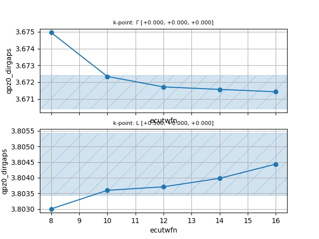
On the basis of this convergence study, we can safely use ecutwfn = 10.
Since we will continue using tgwr_3.abi to perform other convergence studies,
it is a good idea to move the previously generated GWR.nc files and the python script
to a new directory to avoid overlaps between different calculations.
You can, for example, use the following list of shell commands:
mkdir conv_ecutwfn
mv conv_ecutwfn.py conv_ecutwfn
mv tgwr_3o_* log conv_ecutwfn
Convergence wrt nband and ecuteps
To perform a double convergence study in nband and ecuteps,
define a double loop with udtset, and add this section to tgwr_3.abi:
ndtset 16    # NB: ndtset must be equal to udtset[0] * udtset[1]
udtset 4 4

#inner loop: increase nband. The number of iterations is given by udtset[0]
nband:? 150    nband+? 50

#outer loop: increase ecuteps. The number of iterations is given by udtset[1]
ecuteps?: 6     ecuteps?+  2
If we analyze the wall-time required by each dataset, we observe that, at variance with the conventional GW code, the values of nband and ecuteps have little impact of the computational cost.
grep "dataset:" log | grep "<< TIME"
Once the calculation is completed, plot the convergence of the direct QP gaps with the following script:
#!/usr/bin/env python

udtset = [4, 4]  # Should be equal to the grid used in the ABINIT input file

filepaths = [f"tgwr_3o_DS{i}{j}_GWR.nc"
             for i in range(1, udtset[0]+1) for j in range(1, udtset[1]+1)]

from abipy.electrons.gwr import GwrRobot
robot = GwrRobot.from_files(filepaths)

# Convergence window in eV
abs_conv = 0.005

robot.plot_qpgaps_convergence(x="nband",
                              abs_conv=abs_conv, hue="ecuteps",
                              savefig="conv_nband_ecuteps.png",
                              )

robot.plot_qpgaps_convergence(x="ecuteps",
                              abs_conv=abs_conv, hue="nband",
                              savefig="conv_ecuteps_nband.png",
                              )
Again, save the script in a file, let’s say conv_nband_ecuteps.py, in the same
directory where we have launched the calculation, make the file executable and run it with:
./conv_nband_ecuteps.py
You should obtain the following plots:
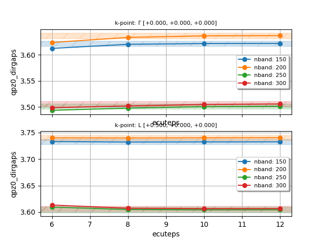
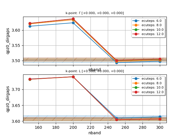
On the basis of this convergence study, we decide to use nband = 250 and ecuteps = 10.
Before proceeding with the next sections, save the results in a different directory by executing:
mkdir conv_nband_ecuteps
mv conv_nband_ecuteps.py conv_nband_ecuteps
mv tgwr_3o_* log conv_nband_ecuteps
Convergence wrt gwr_ntau
Now edit tgwr_3.abi, replace the values of nband and ecuteps found earlier,
and define a new one-dimensional multi-dataset to increase gwr_ntau:
ndtset      15
gwr_ntau:   6         # Number of imaginary-time points
gwr_ntau+   2
Once the calculation is finished, save the script reported below in a file,
let’s say conv_ntau.py, in the same directory where we have launched the calculation,
make it executable with chmod and execute it as usual.
#!/usr/bin/env python
filepaths = [f"tgwr_3o_DS{i}_GWR.nc" for i in range(1, 16)]

from abipy.electrons.gwr import GwrRobot
robot = GwrRobot.from_files(filepaths)

abs_conv = 0.005
robot.plot_qpgaps_convergence(x="gwr_ntau",
                              abs_conv=abs_conv,
                              savefig="conv_ntau.png",
                              )
You should get the following figure:
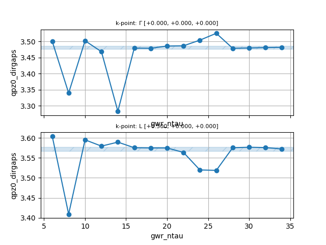
Clearly six minimax points are not enough to convergence.
Also the convergence with gwr_ntau is not variational, and there are meshes that perform better than others.
This study shows that we should use 16-20 minimax points to reach a precision of 0.005 eV (abs_conv).
Unfortunately, this would render the calculations more expensive, especially for a tutorial,
therefore we opt to continue with 12 minimax points for the next calculations.
Again, let’s save the results in a different directory by executing:
mkdir conv_ntau
mv conv_ntau.py conv_ntau
mv tgwr_3o_* log conv_ntau
Convergence wrt gwr_boxcutmin
Now edit tgwr_3.abi, replace the values of nband and ecuteps found earlier,
and define a one-dimensional multidataset to increase gwr_boxcutmin:
ndtset 5
gwr_boxcutmin: 1.1
gwr_boxcutmin+ 0.2
Once the calculation is finished, save the script reported below in a file,
let’s say conv_boxcut.py in the same directory where we launched the calculation,
make it executable and execute it as usual.
#!/usr/bin/env python
filepaths = [f"tgwr_3o_DS{i}_GWR.nc" for i in range(1, 6)]

from abipy.electrons.gwr import GwrRobot
robot = GwrRobot.from_files(filepaths)

abs_conv = 0.005
robot.plot_qpgaps_convergence(x="gwr_boxcutmin",
                              abs_conv=abs_conv,
                              savefig="conv_boxcutmin.png",
                              )
You should obtain the following figure:
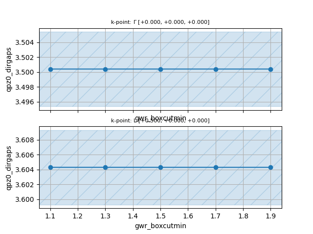
In the case of silicon, the results are rather insensitive to the density of the FFT mesh but keep in mind that other systems may behave differently. We therefore fix gwr_boxcutmin to 1.1.
Note that different values of gwr_boxcutmin can lead to the same value of g_ngfft
as not all the number of points along the three directions of the FFT box are supported by the FFT library.
grep g_ngfft log
g_ngfft: [12, 12, 12, 12, 12, 12, ]
g_ngfft: [15, 15, 15, 15, 15, 15, ]
g_ngfft: [16, 16, 16, 16, 16, 16, ]
g_ngfft: [18, 18, 18, 18, 18, 18, ]
g_ngfft: [20, 20, 20, 20, 20, 20, ]
Note how the wall-time quickly increases with gwr_boxcutmin:
grep "dataset:" log | grep "<< TIME"

 dataset: 1 , wall: 10.75 [s] , cpu: 10.74 [s] <<< TIME
 dataset: 2 , wall: 31.20 [s] , cpu: 31.13 [s] <<< TIME
 dataset: 3 , wall: 50.78 [s] , cpu: 50.68 [s] <<< TIME
 dataset: 4 , wall: 01:27 [minutes] , cpu: 01:27 [minutes] <<< TIME
 dataset: 5 , wall: 02:19 [minutes] , cpu: 02:19 [minutes] <<< TIME
Finally, let’s save the results in a different directory by executing:
mkdir conv_boxcutmin
mv conv_boxcutmin.py conv_boxcutmin
mv tgwr_3o_* log conv_boxcutmin
GWR calculations with different BZ meshes.
In this section of the tutorial, we perform GWR calculations with different BZ meshes. You may want to start immediately the computation by issuing:
mpirun -n 1 tgwr_4.abi > tgwr_4.log 2> err &
with the following input file:
#  Crystalline silicon
#  Calculation of the GW corrections with GWR code and 4x4x4 k-mesh.

# Include geometry and pseudos
include "gwr_include.abi"

################################
# Dataset 3: G0W0 with GWR code
################################
optdriver  6                          # Activate GWR code
ecutwfn    10                         # Truncate basis set when computing G.
                                      # This parameter should be subject to convergence studies
gwr_task "G0W0"                       # One-shot calculation
getden_filepath "tgwr_1o_DS1_DEN"     # Density file


# Definition of the k-point grid
# IMPORTANT: GWR requires Gamma-centered k-meshes
nshiftk 1
shiftk  0.0 0.0 0.0

ngkpt   4 4 4
getwfk_filepath "tgwr_2o_DS2_WFK"       # WFK file with empty states on a 4x4x4 k-mesh

# To perform a convergence study wrt the mesh, comment the two lines above
# and activate the block below.
#ndtset 3
#ngkpt1 2 2 2
#getwfk_filepath1 "tgwr_2o_DS1_WFK"     # WFK file with empty states on a 2x2x2 k-mesh
#ngkpt2 4 4 4
#getwfk_filepath2 "tgwr_2o_DS2_WFK"     # WFK file with empty states on a 4x4x4 k-mesh
#ngkpt3 6 6 6
#getwfk_filepath3 "tgwr_2o_DS3_WFK"     # WFK file with empty states on a 6x6x6 k-mesh

gwr_ntau   12        # Number of imaginary-time points
gwr_boxcutmin  1.0   # This should be subject to convergence studies
gwr_sigma_algo 2     # Use convolutions in the BZ for Sigma

nband      250      # Bands to be used in the screening calculation
ecuteps    10       # Cut-off energy of the planewave set to represent the dielectric matrix.
                    # It is important to adjust this parameter.
#ecutsigx    16     # Dimension of the G sum in Sigma_x.
                    # ecutsigx = ecut is usually a wise choice
                    # (the dimension in Sigma_c is controlled by ecuteps)

nkptgw      2       # number of k-point where to calculate the GW correction
kptgw               # k-points in reduced coordinates
   0.0    0.0    0.0
   0.5    0.0    0.0

bdgw       # calculate GW corrections for bands from 4 to 5
   4  5
   4  5

# Spectral function (very coarse grid to reduce txt file size)
#nfreqsp3 50
#freqspmax3 5 eV

#%%<BEGIN TEST_INFO>
#%% [setup]
#%% executable = abinit
#%% test_chain = tgwr_1.abi, tgwr_2.abi, tgwr_3.abi, tgwr_4.abi, tgwr_5.abi
#%% need_cpp_vars = HAVE_LINALG_SCALAPACK
#%% exclude_builders = eos_nvhpc_23.9_elpa ,eos_nvhpc_24.9_openmpi, haicgu_*
#%% [files]
#%% files_to_test =
#%%   tgwr_4.abo, tolnlines = 25, tolabs = 1.1e-3, tolrel = 3.0e-3, fld_options = -medium;
#%% [paral_info]
#%% max_nprocs = 12
#%% [extra_info]
#%% authors = M. Giantomassi
#%% keywords = NC, GWR
#%% description =
#%%  Crystalline silicon
#%%  Calculation of the GW corrections with GWR code with 4x4x4 k-mesh.
#%%<END TEST_INFO>
The output file is reported here for your convenience:
.Version 10.5.8.2 of ABINIT, released Oct 2025.
.(MPI version, prepared for a x86_64_linux_gnu13.2 computer)
.Copyright (C) 1998-2026 ABINIT group .
ABINIT comes with ABSOLUTELY NO WARRANTY.
It is free software, and you are welcome to redistribute it
under certain conditions (GNU General Public License,
see ~abinit/COPYING or http://www.gnu.org/copyleft/gpl.txt).
ABINIT is a project of the Universite Catholique de Louvain,
Corning Inc. and other collaborators, see ~abinit/doc/developers/contributors.txt .
Please read https://docs.abinit.org/theory/acknowledgments for suggested
acknowledgments of the ABINIT effort.
For more information, see https://www.abinit.org .
.Starting date : Sat 20 Dec 2025.
- ( at 17h07 )
- input file -> /home/buildbot/ABINIT3/eos_gnu_13.2_mpich/trunk__codata2022/tests/TestBot_MPI1/tutorial_tgwr_1-tgwr_2-tgwr_3-tgwr_4-tgwr_5/tgwr_4.abi
- output file -> tgwr_4.abo
- root for input files -> tgwr_4i
- root for output files -> tgwr_4o
Symmetries : space group Fd -3 m (#227); Bravais cF (face-center cubic)
================================================================================
Values of the parameters that define the memory need of the present run
intxc = 0 ionmov = 0 iscf = 7 lmnmax = 6
lnmax = 6 mgfft = 30 mpssoang = 3 mqgrid = 3001
natom = 2 nloc_mem = 1 nspden = 1 nspinor = 1
nsppol = 1 nsym = 48 n1xccc = 2501 ntypat = 1
occopt = 1 xclevel = 2
- mband = 250 mffmem = 1 mkmem = 8
mpw = 848 nfft = 27000 nkpt = 8
================================================================================
P This job should need less than 36.924 Mbytes of memory.
Rough estimation (10% accuracy) of disk space for files :
_ WF disk file : 25.881 Mbytes ; DEN or POT disk file : 0.208 Mbytes.
================================================================================
--------------------------------------------------------------------------------
------------- Echo of variables that govern the present computation ------------
--------------------------------------------------------------------------------
-
- outvars: echo of selected default values
- iomode0 = 0 , fftalg0 =512 , wfoptalg0 = 0
-
- outvars: echo of global parameters not present in the input file
- max_nthreads = 0
-
-outvars: echo values of preprocessed input variables --------
acell 1.0260000000E+01 1.0260000000E+01 1.0260000000E+01 Bohr
amu 2.80855000E+01
bdgw 4 5 4 5
ecut 1.60000000E+01 Hartree
ecuteps 1.00000000E+01 Hartree
ecutsigx 1.60000000E+01 Hartree
ecutwfn 1.00000000E+01 Hartree
- fftalg 512
gwr_sigma_algo 2
istwfk 2 0 3 0 0 0 7 0
ixc 11
kpt 0.00000000E+00 0.00000000E+00 0.00000000E+00
2.50000000E-01 0.00000000E+00 0.00000000E+00
5.00000000E-01 0.00000000E+00 0.00000000E+00
2.50000000E-01 2.50000000E-01 0.00000000E+00
5.00000000E-01 2.50000000E-01 0.00000000E+00
-2.50000000E-01 2.50000000E-01 0.00000000E+00
5.00000000E-01 5.00000000E-01 0.00000000E+00
-2.50000000E-01 5.00000000E-01 2.50000000E-01
kptgw 0.00000000E+00 0.00000000E+00 0.00000000E+00
5.00000000E-01 0.00000000E+00 0.00000000E+00
kptrlatt 4 0 0 0 4 0 0 0 4
kptrlen 2.90196623E+01
P mkmem 8
natom 2
nband 250
ngfft 30 30 30
nkpt 8
nkptgw 2
nsym 48
ntypat 1
occ 2.000000 2.000000 2.000000 2.000000 0.000000 0.000000
0.000000 0.000000 0.000000 0.000000 0.000000 0.000000
0.000000 0.000000 0.000000 0.000000 0.000000 0.000000
0.000000 0.000000 0.000000 0.000000 0.000000 0.000000
0.000000 0.000000 0.000000 0.000000 0.000000 0.000000
0.000000 0.000000 0.000000 0.000000 0.000000 0.000000
0.000000 0.000000 0.000000 0.000000 0.000000 0.000000
0.000000 0.000000 0.000000 0.000000 0.000000 0.000000
0.000000 0.000000 0.000000 0.000000 0.000000 0.000000
0.000000 0.000000 0.000000 0.000000 0.000000 0.000000
0.000000 0.000000 0.000000 0.000000 0.000000 0.000000
0.000000 0.000000 0.000000 0.000000 0.000000 0.000000
0.000000 0.000000 0.000000 0.000000 0.000000 0.000000
0.000000 0.000000 0.000000 0.000000 0.000000 0.000000
0.000000 0.000000 0.000000 0.000000 0.000000 0.000000
0.000000 0.000000 0.000000 0.000000 0.000000 0.000000
0.000000 0.000000 0.000000 0.000000 0.000000 0.000000
0.000000 0.000000 0.000000 0.000000 0.000000 0.000000
0.000000 0.000000 0.000000 0.000000 0.000000 0.000000
0.000000 0.000000 0.000000 0.000000 0.000000 0.000000
0.000000 0.000000 0.000000 0.000000 0.000000 0.000000
0.000000 0.000000 0.000000 0.000000 0.000000 0.000000
0.000000 0.000000 0.000000 0.000000 0.000000 0.000000
0.000000 0.000000 0.000000 0.000000 0.000000 0.000000
0.000000 0.000000 0.000000 0.000000 0.000000 0.000000
0.000000 0.000000 0.000000 0.000000 0.000000 0.000000
0.000000 0.000000 0.000000 0.000000 0.000000 0.000000
0.000000 0.000000 0.000000 0.000000 0.000000 0.000000
0.000000 0.000000 0.000000 0.000000 0.000000 0.000000
0.000000 0.000000 0.000000 0.000000 0.000000 0.000000
0.000000 0.000000 0.000000 0.000000 0.000000 0.000000
0.000000 0.000000 0.000000 0.000000 0.000000 0.000000
0.000000 0.000000 0.000000 0.000000 0.000000 0.000000
0.000000 0.000000 0.000000 0.000000 0.000000 0.000000
0.000000 0.000000 0.000000 0.000000 0.000000 0.000000
0.000000 0.000000 0.000000 0.000000 0.000000 0.000000
0.000000 0.000000 0.000000 0.000000 0.000000 0.000000
0.000000 0.000000 0.000000 0.000000 0.000000 0.000000
0.000000 0.000000 0.000000 0.000000 0.000000 0.000000
0.000000 0.000000 0.000000 0.000000 0.000000 0.000000
0.000000 0.000000 0.000000 0.000000 0.000000 0.000000
0.000000 0.000000 0.000000 0.000000
optdriver 6
rprim 0.0000000000E+00 5.0000000000E-01 5.0000000000E-01
5.0000000000E-01 0.0000000000E+00 5.0000000000E-01
5.0000000000E-01 5.0000000000E-01 0.0000000000E+00
spgroup 227
symrel 1 0 0 0 1 0 0 0 1 -1 0 0 0 -1 0 0 0 -1
0 -1 1 0 -1 0 1 -1 0 0 1 -1 0 1 0 -1 1 0
-1 0 0 -1 0 1 -1 1 0 1 0 0 1 0 -1 1 -1 0
0 1 -1 1 0 -1 0 0 -1 0 -1 1 -1 0 1 0 0 1
-1 0 0 -1 1 0 -1 0 1 1 0 0 1 -1 0 1 0 -1
0 -1 1 1 -1 0 0 -1 0 0 1 -1 -1 1 0 0 1 0
1 0 0 0 0 1 0 1 0 -1 0 0 0 0 -1 0 -1 0
0 1 -1 0 0 -1 1 0 -1 0 -1 1 0 0 1 -1 0 1
-1 0 1 -1 1 0 -1 0 0 1 0 -1 1 -1 0 1 0 0
0 -1 0 1 -1 0 0 -1 1 0 1 0 -1 1 0 0 1 -1
1 0 -1 0 0 -1 0 1 -1 -1 0 1 0 0 1 0 -1 1
0 1 0 0 0 1 1 0 0 0 -1 0 0 0 -1 -1 0 0
1 0 -1 0 1 -1 0 0 -1 -1 0 1 0 -1 1 0 0 1
0 -1 0 0 -1 1 1 -1 0 0 1 0 0 1 -1 -1 1 0
-1 0 1 -1 0 0 -1 1 0 1 0 -1 1 0 0 1 -1 0
0 1 0 1 0 0 0 0 1 0 -1 0 -1 0 0 0 0 -1
0 0 -1 0 1 -1 1 0 -1 0 0 1 0 -1 1 -1 0 1
1 -1 0 0 -1 1 0 -1 0 -1 1 0 0 1 -1 0 1 0
0 0 1 1 0 0 0 1 0 0 0 -1 -1 0 0 0 -1 0
-1 1 0 -1 0 0 -1 0 1 1 -1 0 1 0 0 1 0 -1
0 0 1 0 1 0 1 0 0 0 0 -1 0 -1 0 -1 0 0
1 -1 0 0 -1 0 0 -1 1 -1 1 0 0 1 0 0 1 -1
0 0 -1 1 0 -1 0 1 -1 0 0 1 -1 0 1 0 -1 1
-1 1 0 -1 0 1 -1 0 0 1 -1 0 1 0 -1 1 0 0
tnons 0.0000000 0.0000000 0.0000000 0.2500000 0.2500000 0.2500000
0.0000000 0.0000000 0.0000000 0.2500000 0.2500000 0.2500000
0.0000000 0.0000000 0.0000000 0.2500000 0.2500000 0.2500000
0.0000000 0.0000000 0.0000000 0.2500000 0.2500000 0.2500000
0.0000000 0.0000000 0.0000000 0.2500000 0.2500000 0.2500000
0.0000000 0.0000000 0.0000000 0.2500000 0.2500000 0.2500000
0.0000000 0.0000000 0.0000000 0.2500000 0.2500000 0.2500000
0.0000000 0.0000000 0.0000000 0.2500000 0.2500000 0.2500000
0.0000000 0.0000000 0.0000000 0.2500000 0.2500000 0.2500000
0.0000000 0.0000000 0.0000000 0.2500000 0.2500000 0.2500000
0.0000000 0.0000000 0.0000000 0.2500000 0.2500000 0.2500000
0.0000000 0.0000000 0.0000000 0.2500000 0.2500000 0.2500000
0.0000000 0.0000000 0.0000000 0.2500000 0.2500000 0.2500000
0.0000000 0.0000000 0.0000000 0.2500000 0.2500000 0.2500000
0.0000000 0.0000000 0.0000000 0.2500000 0.2500000 0.2500000
0.0000000 0.0000000 0.0000000 0.2500000 0.2500000 0.2500000
0.0000000 0.0000000 0.0000000 0.2500000 0.2500000 0.2500000
0.0000000 0.0000000 0.0000000 0.2500000 0.2500000 0.2500000
0.0000000 0.0000000 0.0000000 0.2500000 0.2500000 0.2500000
0.0000000 0.0000000 0.0000000 0.2500000 0.2500000 0.2500000
0.0000000 0.0000000 0.0000000 0.2500000 0.2500000 0.2500000
0.0000000 0.0000000 0.0000000 0.2500000 0.2500000 0.2500000
0.0000000 0.0000000 0.0000000 0.2500000 0.2500000 0.2500000
0.0000000 0.0000000 0.0000000 0.2500000 0.2500000 0.2500000
typat 1 1
wtk 0.01563 0.12500 0.06250 0.09375 0.37500 0.18750
0.04688 0.09375
xangst 0.0000000000E+00 0.0000000000E+00 0.0000000000E+00
1.3573395450E+00 1.3573395450E+00 1.3573395450E+00
xcart 0.0000000000E+00 0.0000000000E+00 0.0000000000E+00
2.5650000000E+00 2.5650000000E+00 2.5650000000E+00
xred 0.0000000000E+00 0.0000000000E+00 0.0000000000E+00
2.5000000000E-01 2.5000000000E-01 2.5000000000E-01
znucl 14.00000
================================================================================
chkinp: Checking input parameters for consistency.
================================================================================
== DATASET 1 ==================================================================
- mpi_nproc: 1, omp_nthreads: -1 (-1 if OMP is not activated)
--- !DatasetInfo
iteration_state: {dtset: 1, }
dimensions: {natom: 2, nkpt: 8, mband: 250, nsppol: 1, nspinor: 1, nspden: 1, mpw: 848, }
cutoff_energies: {ecut: 16.0, pawecutdg: -1.0, }
electrons: {nelect: 8.00000000E+00, charge: 0.00000000E+00, occopt: 1.00000000E+00, tsmear: 1.00000000E-02, }
meta: {optdriver: 6, }
...
mkfilename: getwfk from: tgwr_2o_DS2_WFK
mkfilename: getden from: tgwr_1o_DS1_DEN
Exchange-correlation functional for the present dataset will be:
GGA: Perdew-Burke-Ernzerhof functional - ixc=11
Citation for XC functional:
J.P.Perdew, K.Burke, M.Ernzerhof, PRL 77, 3865 (1996)
.Using double precision arithmetic; gwpc = 8
- Reading GS density from: tgwr_1o_DS1_DEN
--- Pseudopotential description ------------------------------------------------
- pspini: atom type 1 psp file is /home/buildbot/ABINIT3/eos_gnu_13.2_mpich/trunk__codata2022/tests/Pspdir/Psdj_nc_sr_04_pbe_std_psp8/Si.psp8
- pspatm: opening atomic psp file /home/buildbot/ABINIT3/eos_gnu_13.2_mpich/trunk__codata2022/tests/Pspdir/Psdj_nc_sr_04_pbe_std_psp8/Si.psp8
- Si ONCVPSP-3.2.3.1 r_core= 1.60303 1.72197 1.91712
- 14.00000 4.00000 170510 znucl, zion, pspdat
8 11 2 4 600 0.00000 pspcod,pspxc,lmax,lloc,mmax,r2well
5.99000000000000 4.00000000000000 0.00000000000000 rchrg,fchrg,qchrg
nproj 2 2 2
extension_switch 1
pspatm : epsatm= 9.34321699
--- l ekb(1:nproj) -->
0 5.168965 0.829883
1 2.571282 0.578307
2 -2.427311 -0.488097
pspatm: atomic psp has been read and splines computed
1.49491472E+02 ecore*ucvol(ha*bohr**3)
--------------------------------------------------------------------------------
Total charge density [el/Bohr^3]
) Maximum= 8.5569E-02 at reduced coord. 0.1000 0.1000 0.7000
) Minimum= 1.4870E-03 at reduced coord. 0.0000 0.0000 0.0000
Integrated= 8.0000E+00
- Reading GS states from WFK file: tgwr_2o_DS2_WFK
Mapping kBZ --> kIBZ
Legend: bz = TS(ibz) + g0 where isym is the index of the symrec operation S and itim is 1 if TR is used.
BZ IBZ ibz isym itim g0
1 [ 0.0000E+00, 0.0000E+00, 0.0000E+00] [ 0.0000E+00, 0.0000E+00, 0.0000E+00] 1 1 0 [0, 0, 0]
2 [ 2.5000E-01, 0.0000E+00, 0.0000E+00] [ 2.5000E-01, 0.0000E+00, 0.0000E+00] 2 1 0 [0, 0, 0]
3 [-2.5000E-01, -2.5000E-01, -2.5000E-01] [ 2.5000E-01, 0.0000E+00, 0.0000E+00] 2 5 0 [0, 0, 0]
4 [ 0.0000E+00, 2.5000E-01, 0.0000E+00] [ 2.5000E-01, 0.0000E+00, 0.0000E+00] 2 7 0 [0, 0, 0]
5 [ 0.0000E+00, 0.0000E+00, 2.5000E-01] [ 2.5000E-01, 0.0000E+00, 0.0000E+00] 2 3 0 [0, 0, 0]
6 [ 0.0000E+00, -2.5000E-01, 0.0000E+00] [ 2.5000E-01, 0.0000E+00, 0.0000E+00] 2 8 0 [0, 0, 0]
7 [-2.5000E-01, 0.0000E+00, 0.0000E+00] [ 2.5000E-01, 0.0000E+00, 0.0000E+00] 2 2 0 [0, 0, 0]
8 [ 0.0000E+00, 0.0000E+00, -2.5000E-01] [ 2.5000E-01, 0.0000E+00, 0.0000E+00] 2 4 0 [0, 0, 0]
9 [ 2.5000E-01, 2.5000E-01, 2.5000E-01] [ 2.5000E-01, 0.0000E+00, 0.0000E+00] 2 6 0 [0, 0, 0]
10 [ 5.0000E-01, 0.0000E+00, 0.0000E+00] [ 5.0000E-01, 0.0000E+00, 0.0000E+00] 3 1 0 [0, 0, 0]
11 [ 5.0000E-01, 5.0000E-01, 5.0000E-01] [ 5.0000E-01, 0.0000E+00, 0.0000E+00] 3 5 0 [1, 1, 1]
12 [ 0.0000E+00, 0.0000E+00, 5.0000E-01] [ 5.0000E-01, 0.0000E+00, 0.0000E+00] 3 3 0 [0, 0, 0]
13 [ 0.0000E+00, 5.0000E-01, 0.0000E+00] [ 5.0000E-01, 0.0000E+00, 0.0000E+00] 3 7 0 [0, 0, 0]
14 [ 2.5000E-01, 2.5000E-01, 0.0000E+00] [ 2.5000E-01, 2.5000E-01, 0.0000E+00] 4 1 0 [0, 0, 0]
15 [ 0.0000E+00, 2.5000E-01, 2.5000E-01] [ 2.5000E-01, 2.5000E-01, 0.0000E+00] 4 17 0 [0, 0, 0]
16 [ 0.0000E+00, -2.5000E-01, -2.5000E-01] [ 2.5000E-01, 2.5000E-01, 0.0000E+00] 4 18 0 [0, 0, 0]
17 [ 2.5000E-01, 0.0000E+00, 2.5000E-01] [ 2.5000E-01, 2.5000E-01, 0.0000E+00] 4 10 0 [0, 0, 0]
18 [-2.5000E-01, 0.0000E+00, -2.5000E-01] [ 2.5000E-01, 2.5000E-01, 0.0000E+00] 4 9 0 [0, 0, 0]
19 [-2.5000E-01, -2.5000E-01, 0.0000E+00] [ 2.5000E-01, 2.5000E-01, 0.0000E+00] 4 2 0 [0, 0, 0]
20 [ 5.0000E-01, 2.5000E-01, 0.0000E+00] [ 5.0000E-01, 2.5000E-01, 0.0000E+00] 5 1 0 [0, 0, 0]
prtvol = 0, max 20 points are written
Mapping qBZ --> qIBZ
Legend: bz = TS(ibz) + g0 where isym is the index of the symrec operation S and itim is 1 if TR is used.
BZ IBZ ibz isym itim g0
1 [ 0.0000E+00, 0.0000E+00, 0.0000E+00] [ 0.0000E+00, 0.0000E+00, 0.0000E+00] 1 1 0 [0, 0, 0]
2 [ 2.5000E-01, 0.0000E+00, 0.0000E+00] [ 2.5000E-01, 0.0000E+00, 0.0000E+00] 2 1 0 [0, 0, 0]
3 [-2.5000E-01, -2.5000E-01, -2.5000E-01] [ 2.5000E-01, 0.0000E+00, 0.0000E+00] 2 5 0 [0, 0, 0]
4 [ 0.0000E+00, 2.5000E-01, 0.0000E+00] [ 2.5000E-01, 0.0000E+00, 0.0000E+00] 2 7 0 [0, 0, 0]
5 [ 0.0000E+00, 0.0000E+00, 2.5000E-01] [ 2.5000E-01, 0.0000E+00, 0.0000E+00] 2 3 0 [0, 0, 0]
6 [ 0.0000E+00, -2.5000E-01, 0.0000E+00] [ 2.5000E-01, 0.0000E+00, 0.0000E+00] 2 8 0 [0, 0, 0]
7 [-2.5000E-01, 0.0000E+00, 0.0000E+00] [ 2.5000E-01, 0.0000E+00, 0.0000E+00] 2 2 0 [0, 0, 0]
8 [ 0.0000E+00, 0.0000E+00, -2.5000E-01] [ 2.5000E-01, 0.0000E+00, 0.0000E+00] 2 4 0 [0, 0, 0]
9 [ 2.5000E-01, 2.5000E-01, 2.5000E-01] [ 2.5000E-01, 0.0000E+00, 0.0000E+00] 2 6 0 [0, 0, 0]
10 [ 5.0000E-01, 0.0000E+00, 0.0000E+00] [ 5.0000E-01, 0.0000E+00, 0.0000E+00] 3 1 0 [0, 0, 0]
11 [ 5.0000E-01, 5.0000E-01, 5.0000E-01] [ 5.0000E-01, 0.0000E+00, 0.0000E+00] 3 5 0 [1, 1, 1]
12 [ 0.0000E+00, 0.0000E+00, 5.0000E-01] [ 5.0000E-01, 0.0000E+00, 0.0000E+00] 3 3 0 [0, 0, 0]
13 [ 0.0000E+00, 5.0000E-01, 0.0000E+00] [ 5.0000E-01, 0.0000E+00, 0.0000E+00] 3 7 0 [0, 0, 0]
14 [ 2.5000E-01, 2.5000E-01, 0.0000E+00] [ 2.5000E-01, 2.5000E-01, 0.0000E+00] 4 1 0 [0, 0, 0]
15 [ 0.0000E+00, 2.5000E-01, 2.5000E-01] [ 2.5000E-01, 2.5000E-01, 0.0000E+00] 4 17 0 [0, 0, 0]
16 [ 0.0000E+00, -2.5000E-01, -2.5000E-01] [ 2.5000E-01, 2.5000E-01, 0.0000E+00] 4 18 0 [0, 0, 0]
17 [ 2.5000E-01, 0.0000E+00, 2.5000E-01] [ 2.5000E-01, 2.5000E-01, 0.0000E+00] 4 10 0 [0, 0, 0]
18 [-2.5000E-01, 0.0000E+00, -2.5000E-01] [ 2.5000E-01, 2.5000E-01, 0.0000E+00] 4 9 0 [0, 0, 0]
19 [-2.5000E-01, -2.5000E-01, 0.0000E+00] [ 2.5000E-01, 2.5000E-01, 0.0000E+00] 4 2 0 [0, 0, 0]
20 [ 5.0000E-01, 2.5000E-01, 0.0000E+00] [ 5.0000E-01, 2.5000E-01, 0.0000E+00] 5 1 0 [0, 0, 0]
prtvol = 0, max 20 points are written
=== Kohn-Sham gaps and band edges from IBZ mesh ===
Indirect band gap semiconductor
Fundamental gap: 0.707 (eV)
VBM: -0.354 (eV) at k: [ 0.0000E+00, 0.0000E+00, 0.0000E+00]
CBM: 0.354 (eV) at k: [ 5.0000E-01, 5.0000E-01, 0.0000E+00]
Direct gap: 2.556 (eV) at k: [ 0.0000E+00, 0.0000E+00, 0.0000E+00]
- Optimizing MPI grid with mem_per_cpu_mb: 2.048000E+03 [Mb]
- Use `abinit run.abi --mem-per-cpu=4G` to set mem_per_cpu_mb in the submission script
- np_k np_g np_t np_s memb_per_cpu efficiency speedup
- 1 1 1 1 3.37502E+03 1.00000E+00 1.00000E+00
-
- Selected MPI grid:
- np_k np_g np_t np_s memb_per_cpu efficiency speedup
- 1 1 1 1 3.37502E+03 1.00000E+00 1.00000E+00
- Resident memory in Mb for G(g,g',+/-tau) and chi(g,g',tau):
- G_k(g,g,tau): 1009.1
- Chi_q(g,g,tau): 252.3
- u_k(g,b): 12.7
- Temporary memory allocated inside the tau loops:
- G_k(r,g): 1400.6
- chi_q(r,g): 700.3
P kpt_comm can use shmem: yes
P g_comm can use shmem: yes
P tau_comm can use shmem: yes
P spin_comm can use shmem yes
- FFT uc_batch_size: 1
- FFT sc_batch_size: 1
==== Info on the gwr_t object ====
--- !GWR_params
iteration_state: {dtset: 1, }
gwr_task: G0W0
nband: 250
ntau: 12
ngkpt: [4, 4, 4, ]
ngqpt: [4, 4, 4, ]
chi_algo: supercell
sigma_algo: 'BZ-convolutions'
nkibz: 8
nqibz: 8
inclvkb: 2
q0: [ 1.00000000E-05, 2.00000000E-05, 3.00000000E-05, ]
gw_icutcoul: 6
green_mpw: 415
tchi_mpw: 415
g_ngfft: [12, 12, 12, 12, 12, 12, ]
gwr_boxcutmin: 1.00000000E+00
P gwr_np_kgts: [1, 1, 1, 1, ]
P np_kibz: [1, 1, 1, 1, 1, 1, 1, 1, ]
P np_qibz: [1, 1, 1, 1, 1, 1, 1, 1, ]
min_transition_energy_eV: 7.07322783E-01
max_transition_energy_eV: 1.92973205E+02
eratio: 2.72821984E+02
ft_max_err_t2w_cos: 1.19236269E-03
ft_max_err_w2t_cos: 3.51829949E-05
ft_max_err_t2w_sin: 2.27332971E-02
cosft_duality_error: 4.80114081E-03
Minimax imaginary tau/omega mesh in a.u.: !Tabular | # tau, weight(tau), omega, weight(omega)
1 3.01845E-02 7.84567E-02 6.37107E-03 1.30197E-02
2 1.68348E-01 2.04750E-01 2.08408E-02 1.65798E-02
3 4.62515E-01 4.00892E-01 4.11428E-02 2.50342E-02
4 1.02120E+00 7.51969E-01 7.35654E-02 4.15594E-02
5 2.06352E+00 1.39686E+00 1.29029E-01 7.25879E-02
6 3.98516E+00 2.55709E+00 2.27719E-01 1.30961E-01
7 7.46798E+00 4.59587E+00 4.08469E-01 2.42767E-01
8 1.36656E+01 8.11373E+00 7.48639E-01 4.62721E-01
9 2.45159E+01 1.41167E+01 1.40860E+00 9.11790E-01
10 4.33066E+01 2.43993E+01 2.74298E+00 1.88995E+00
11 7.59655E+01 4.28466E+01 5.67129E+00 4.41801E+00
12 1.35795E+02 8.33674E+01 1.41554E+01 1.63699E+01
...
Cutting u(g) as ecutwfn: 1.000000E+01 < ecut: 1.600000E+01
Computing chi0 head and wings with inclvkb: 2
Using KS orbitals and KS energies...
Computing diagonal matrix elements of Sigma_x
=== Info on Coulomb term used in Sigma_x ===
cutoff-mode = AUXILIARY_FUNCTION
Using KS orbitals and KS energies...
Building Green's functions from KS orbitals and KS energies...
Building correlated screening Wc(i omega) ...
=== Info on Coulomb term used in epsilon and W ===
cutoff-mode = AUXILIARY_FUNCTION
--- !EMACRO_WITHOUT_LOCAL_FIELDS
iteration_state: {dtset: 1, }
'epsilon_{iw, q -> Gamma}(0,0)': !Tabular |
6.37106624E-03 2.40438756E+01 3.38555137E-18
2.08407959E-02 2.34176150E+01 -1.63526676E-17
4.11427666E-02 2.16496344E+01 -6.22745334E-18
7.35653993E-02 1.78507293E+01 1.23414017E-17
1.29029157E-01 1.20491202E+01 1.08577441E-18
2.27718878E-01 6.50362270E+00 -1.65075386E-18
4.08469196E-01 3.16498220E+00 1.32870842E-19
7.48638937E-01 1.72362216E+00 1.51351936E-20
1.40860376E+00 1.21615828E+00 1.04025838E-19
2.74297741E+00 1.05875854E+00 -2.64741174E-20
5.67129327E+00 1.01399671E+00 6.76183000E-21
1.41553560E+01 1.00226743E+00 9.42074914E-22
...
--- !EMACRO_WITH_LOCAL_FIELDS
iteration_state: {dtset: 1, }
'epsilon_{iw, q -> Gamma}(0,0)': !Tabular |
6.37106624E-03 4.57058785E-02 0.00000000E+00
2.08407959E-02 4.68755937E-02 0.00000000E+00
4.11427666E-02 5.05398352E-02 0.00000000E+00
7.35653993E-02 6.08427808E-02 0.00000000E+00
1.29029157E-01 8.89379969E-02 0.00000000E+00
2.27718878E-01 1.61726602E-01 0.00000000E+00
4.08469196E-01 3.25250315E-01 0.00000000E+00
7.48638937E-01 5.86358921E-01 0.00000000E+00
1.40860376E+00 8.24055047E-01 0.00000000E+00
2.74297741E+00 9.44758279E-01 0.00000000E+00
5.67129327E+00 9.86216814E-01 0.00000000E+00
1.41553560E+01 9.97738319E-01 0.00000000E+00
...
Computing diagonal matrix elements of Sigma_c
=== Info on Coulomb term used in Sigma_c ===
cutoff-mode = AUXILIARY_FUNCTION
Building Sigma_c with convolutions in k-space:
================================================================================
QP results (energies in eV)
Notations:
E0: Kohn-Sham energy
<VxcDFT>: Matrix elements of Vxc[n_val] without non-linear core correction (if any)
SigX: Matrix elements of Sigma_x
SigC(E0): Matrix elements of Sigma_c at E0
Z: Renormalization factor
E-E0: Difference between the QP and the KS energy.
E-Eprev: Difference between QP energy at iteration i and i-1
E: Quasi-particle energy
Occ(E): Occupancy of QP state
--- !GWR_SelfEnergy_ee
iteration_state: {dtset: 1, }
kpoint : [ 0.000, 0.000, 0.000, ]
spin : 1
gwr_scf_iteration: 1
gwr_task : G0W0
QP_VBM_band: 4
QP_CBM_band: 5
KS_gap : 2.556
QP_gap : 3.247
Delta_QP_KS: 0.691
data: !Tabular |
Band E0 <VxcDFT> SigX SigC(E0) Z E-E0 E-Eprev E Occ(E)
2 -0.354 -11.319 -13.047 0.743 0.755 -0.743 -0.743 -1.097 2.000
3 -0.354 -11.319 -13.047 0.743 0.755 -0.743 -0.743 -1.097 2.000
4 -0.354 -11.319 -13.047 0.743 0.755 -0.743 -0.743 -1.097 2.000
5 2.202 -10.034 -5.647 -4.456 0.758 -0.052 -0.052 2.150 0.000
6 2.202 -10.034 -5.647 -4.456 0.758 -0.052 -0.052 2.150 0.000
7 2.202 -10.034 -5.647 -4.456 0.758 -0.052 -0.052 2.150 0.000
...
--- !GWR_SelfEnergy_ee
iteration_state: {dtset: 1, }
kpoint : [ 0.500, 0.000, 0.000, ]
spin : 1
gwr_scf_iteration: 1
gwr_task : G0W0
QP_VBM_band: 4
QP_CBM_band: 5
KS_gap : 2.733
QP_gap : 3.413
Delta_QP_KS: 0.680
data: !Tabular |
Band E0 <VxcDFT> SigX SigC(E0) Z E-E0 E-Eprev E Occ(E)
3 -1.556 -11.058 -13.246 1.202 0.749 -0.738 -0.738 -2.294 2.000
4 -1.556 -11.058 -13.246 1.202 0.749 -0.738 -0.738 -2.294 2.000
5 1.177 -10.088 -5.834 -4.330 0.764 -0.058 -0.058 1.119 0.000
...
=== Kohn-Sham gaps and band edges from IBZ mesh ===
Indirect band gap semiconductor
Fundamental gap: 0.707 (eV)
VBM: -0.354 (eV) at k: [ 0.0000E+00, 0.0000E+00, 0.0000E+00]
CBM: 0.354 (eV) at k: [ 5.0000E-01, 5.0000E-01, 0.0000E+00]
Direct gap: 2.556 (eV) at k: [ 0.0000E+00, 0.0000E+00, 0.0000E+00]
=== QP gaps and band edges taking into account Sigma_nk corrections for 2 k-points ===
Indirect band gap semiconductor
Fundamental gap: 1.450 (eV)
VBM: -1.097 (eV) at k: [ 0.0000E+00, 0.0000E+00, 0.0000E+00]
CBM: 0.354 (eV) at k: [ 5.0000E-01, 5.0000E-01, 0.0000E+00]
Direct gap: 2.784 (eV) at k: [ 2.5000E-01, 0.0000E+00, 0.0000E+00]
== END DATASET(S) ==============================================================
================================================================================
-outvars: echo values of variables after computation --------
acell 1.0260000000E+01 1.0260000000E+01 1.0260000000E+01 Bohr
amu 2.80855000E+01
bdgw 4 5 4 5
ecut 1.60000000E+01 Hartree
ecuteps 1.00000000E+01 Hartree
ecutsigx 1.60000000E+01 Hartree
ecutwfn 1.00000000E+01 Hartree
etotal 0.0000000000E+00
fcart 0.0000000000E+00 0.0000000000E+00 0.0000000000E+00
0.0000000000E+00 0.0000000000E+00 0.0000000000E+00
- fftalg 512
gwr_sigma_algo 2
istwfk 2 0 3 0 0 0 7 0
ixc 11
kpt 0.00000000E+00 0.00000000E+00 0.00000000E+00
2.50000000E-01 0.00000000E+00 0.00000000E+00
5.00000000E-01 0.00000000E+00 0.00000000E+00
2.50000000E-01 2.50000000E-01 0.00000000E+00
5.00000000E-01 2.50000000E-01 0.00000000E+00
-2.50000000E-01 2.50000000E-01 0.00000000E+00
5.00000000E-01 5.00000000E-01 0.00000000E+00
-2.50000000E-01 5.00000000E-01 2.50000000E-01
kptgw 0.00000000E+00 0.00000000E+00 0.00000000E+00
5.00000000E-01 0.00000000E+00 0.00000000E+00
kptrlatt 4 0 0 0 4 0 0 0 4
kptrlen 2.90196623E+01
P mkmem 8
natom 2
nband 250
ngfft 30 30 30
nkpt 8
nkptgw 2
nsym 48
ntypat 1
occ 2.000000 2.000000 2.000000 2.000000 0.000000 0.000000
0.000000 0.000000 0.000000 0.000000 0.000000 0.000000
0.000000 0.000000 0.000000 0.000000 0.000000 0.000000
0.000000 0.000000 0.000000 0.000000 0.000000 0.000000
0.000000 0.000000 0.000000 0.000000 0.000000 0.000000
0.000000 0.000000 0.000000 0.000000 0.000000 0.000000
0.000000 0.000000 0.000000 0.000000 0.000000 0.000000
0.000000 0.000000 0.000000 0.000000 0.000000 0.000000
0.000000 0.000000 0.000000 0.000000 0.000000 0.000000
0.000000 0.000000 0.000000 0.000000 0.000000 0.000000
0.000000 0.000000 0.000000 0.000000 0.000000 0.000000
0.000000 0.000000 0.000000 0.000000 0.000000 0.000000
0.000000 0.000000 0.000000 0.000000 0.000000 0.000000
0.000000 0.000000 0.000000 0.000000 0.000000 0.000000
0.000000 0.000000 0.000000 0.000000 0.000000 0.000000
0.000000 0.000000 0.000000 0.000000 0.000000 0.000000
0.000000 0.000000 0.000000 0.000000 0.000000 0.000000
0.000000 0.000000 0.000000 0.000000 0.000000 0.000000
0.000000 0.000000 0.000000 0.000000 0.000000 0.000000
0.000000 0.000000 0.000000 0.000000 0.000000 0.000000
0.000000 0.000000 0.000000 0.000000 0.000000 0.000000
0.000000 0.000000 0.000000 0.000000 0.000000 0.000000
0.000000 0.000000 0.000000 0.000000 0.000000 0.000000
0.000000 0.000000 0.000000 0.000000 0.000000 0.000000
0.000000 0.000000 0.000000 0.000000 0.000000 0.000000
0.000000 0.000000 0.000000 0.000000 0.000000 0.000000
0.000000 0.000000 0.000000 0.000000 0.000000 0.000000
0.000000 0.000000 0.000000 0.000000 0.000000 0.000000
0.000000 0.000000 0.000000 0.000000 0.000000 0.000000
0.000000 0.000000 0.000000 0.000000 0.000000 0.000000
0.000000 0.000000 0.000000 0.000000 0.000000 0.000000
0.000000 0.000000 0.000000 0.000000 0.000000 0.000000
0.000000 0.000000 0.000000 0.000000 0.000000 0.000000
0.000000 0.000000 0.000000 0.000000 0.000000 0.000000
0.000000 0.000000 0.000000 0.000000 0.000000 0.000000
0.000000 0.000000 0.000000 0.000000 0.000000 0.000000
0.000000 0.000000 0.000000 0.000000 0.000000 0.000000
0.000000 0.000000 0.000000 0.000000 0.000000 0.000000
0.000000 0.000000 0.000000 0.000000 0.000000 0.000000
0.000000 0.000000 0.000000 0.000000 0.000000 0.000000
0.000000 0.000000 0.000000 0.000000 0.000000 0.000000
0.000000 0.000000 0.000000 0.000000
optdriver 6
rprim 0.0000000000E+00 5.0000000000E-01 5.0000000000E-01
5.0000000000E-01 0.0000000000E+00 5.0000000000E-01
5.0000000000E-01 5.0000000000E-01 0.0000000000E+00
spgroup 227
strten 0.0000000000E+00 0.0000000000E+00 0.0000000000E+00
0.0000000000E+00 0.0000000000E+00 0.0000000000E+00
symrel 1 0 0 0 1 0 0 0 1 -1 0 0 0 -1 0 0 0 -1
0 -1 1 0 -1 0 1 -1 0 0 1 -1 0 1 0 -1 1 0
-1 0 0 -1 0 1 -1 1 0 1 0 0 1 0 -1 1 -1 0
0 1 -1 1 0 -1 0 0 -1 0 -1 1 -1 0 1 0 0 1
-1 0 0 -1 1 0 -1 0 1 1 0 0 1 -1 0 1 0 -1
0 -1 1 1 -1 0 0 -1 0 0 1 -1 -1 1 0 0 1 0
1 0 0 0 0 1 0 1 0 -1 0 0 0 0 -1 0 -1 0
0 1 -1 0 0 -1 1 0 -1 0 -1 1 0 0 1 -1 0 1
-1 0 1 -1 1 0 -1 0 0 1 0 -1 1 -1 0 1 0 0
0 -1 0 1 -1 0 0 -1 1 0 1 0 -1 1 0 0 1 -1
1 0 -1 0 0 -1 0 1 -1 -1 0 1 0 0 1 0 -1 1
0 1 0 0 0 1 1 0 0 0 -1 0 0 0 -1 -1 0 0
1 0 -1 0 1 -1 0 0 -1 -1 0 1 0 -1 1 0 0 1
0 -1 0 0 -1 1 1 -1 0 0 1 0 0 1 -1 -1 1 0
-1 0 1 -1 0 0 -1 1 0 1 0 -1 1 0 0 1 -1 0
0 1 0 1 0 0 0 0 1 0 -1 0 -1 0 0 0 0 -1
0 0 -1 0 1 -1 1 0 -1 0 0 1 0 -1 1 -1 0 1
1 -1 0 0 -1 1 0 -1 0 -1 1 0 0 1 -1 0 1 0
0 0 1 1 0 0 0 1 0 0 0 -1 -1 0 0 0 -1 0
-1 1 0 -1 0 0 -1 0 1 1 -1 0 1 0 0 1 0 -1
0 0 1 0 1 0 1 0 0 0 0 -1 0 -1 0 -1 0 0
1 -1 0 0 -1 0 0 -1 1 -1 1 0 0 1 0 0 1 -1
0 0 -1 1 0 -1 0 1 -1 0 0 1 -1 0 1 0 -1 1
-1 1 0 -1 0 1 -1 0 0 1 -1 0 1 0 -1 1 0 0
tnons 0.0000000 0.0000000 0.0000000 0.2500000 0.2500000 0.2500000
0.0000000 0.0000000 0.0000000 0.2500000 0.2500000 0.2500000
0.0000000 0.0000000 0.0000000 0.2500000 0.2500000 0.2500000
0.0000000 0.0000000 0.0000000 0.2500000 0.2500000 0.2500000
0.0000000 0.0000000 0.0000000 0.2500000 0.2500000 0.2500000
0.0000000 0.0000000 0.0000000 0.2500000 0.2500000 0.2500000
0.0000000 0.0000000 0.0000000 0.2500000 0.2500000 0.2500000
0.0000000 0.0000000 0.0000000 0.2500000 0.2500000 0.2500000
0.0000000 0.0000000 0.0000000 0.2500000 0.2500000 0.2500000
0.0000000 0.0000000 0.0000000 0.2500000 0.2500000 0.2500000
0.0000000 0.0000000 0.0000000 0.2500000 0.2500000 0.2500000
0.0000000 0.0000000 0.0000000 0.2500000 0.2500000 0.2500000
0.0000000 0.0000000 0.0000000 0.2500000 0.2500000 0.2500000
0.0000000 0.0000000 0.0000000 0.2500000 0.2500000 0.2500000
0.0000000 0.0000000 0.0000000 0.2500000 0.2500000 0.2500000
0.0000000 0.0000000 0.0000000 0.2500000 0.2500000 0.2500000
0.0000000 0.0000000 0.0000000 0.2500000 0.2500000 0.2500000
0.0000000 0.0000000 0.0000000 0.2500000 0.2500000 0.2500000
0.0000000 0.0000000 0.0000000 0.2500000 0.2500000 0.2500000
0.0000000 0.0000000 0.0000000 0.2500000 0.2500000 0.2500000
0.0000000 0.0000000 0.0000000 0.2500000 0.2500000 0.2500000
0.0000000 0.0000000 0.0000000 0.2500000 0.2500000 0.2500000
0.0000000 0.0000000 0.0000000 0.2500000 0.2500000 0.2500000
0.0000000 0.0000000 0.0000000 0.2500000 0.2500000 0.2500000
typat 1 1
wtk 0.01563 0.12500 0.06250 0.09375 0.37500 0.18750
0.04688 0.09375
xangst 0.0000000000E+00 0.0000000000E+00 0.0000000000E+00
1.3573395450E+00 1.3573395450E+00 1.3573395450E+00
xcart 0.0000000000E+00 0.0000000000E+00 0.0000000000E+00
2.5650000000E+00 2.5650000000E+00 2.5650000000E+00
xred 0.0000000000E+00 0.0000000000E+00 0.0000000000E+00
2.5000000000E-01 2.5000000000E-01 2.5000000000E-01
znucl 14.00000
================================================================================
- Timing analysis has been suppressed with timopt=0
================================================================================
Suggested references for the acknowledgment of ABINIT usage.
The users of ABINIT have little formal obligations with respect to the ABINIT group
(those specified in the GNU General Public License, http://www.gnu.org/copyleft/gpl.txt).
However, it is common practice in the scientific literature,
to acknowledge the efforts of people that have made the research possible.
In this spirit, please find below suggested citations of work written by ABINIT developers,
corresponding to implementations inside of ABINIT that you have used in the present run.
Note also that it will be of great value to readers of publications presenting these results,
to read papers enabling them to understand the theoretical formalism and details
of the ABINIT implementation.
For information on why they are suggested, see also https://docs.abinit.org/theory/acknowledgments.
-
- [1] The Abinit project: Impact, environment and recent developments.
- Computer Phys. Comm. 248, 107042 (2020).
- X.Gonze, B. Amadon, G. Antonius, F.Arnardi, L.Baguet, J.-M.Beuken,
- J.Bieder, F.Bottin, J.Bouchet, E.Bousquet, N.Brouwer, F.Bruneval,
- G.Brunin, T.Cavignac, J.-B. Charraud, Wei Chen, M.Cote, S.Cottenier,
- J.Denier, G.Geneste, Ph.Ghosez, M.Giantomassi, Y.Gillet, O.Gingras,
- D.R.Hamann, G.Hautier, Xu He, N.Helbig, N.Holzwarth, Y.Jia, F.Jollet,
- W.Lafargue-Dit-Hauret, K.Lejaeghere, M.A.L.Marques, A.Martin, C.Martins,
- H.P.C. Miranda, F.Naccarato, K. Persson, G.Petretto, V.Planes, Y.Pouillon,
- S.Prokhorenko, F.Ricci, G.-M.Rignanese, A.H.Romero, M.M.Schmitt, M.Torrent,
- M.J.van Setten, B.Van Troeye, M.J.Verstraete, G.Zerah and J.W.Zwanzig
- Comment: the fifth generic paper describing the ABINIT project.
- Note that a version of this paper, that is not formatted for Computer Phys. Comm.
- is available at https://www.abinit.org/sites/default/files/ABINIT20.pdf .
- The licence allows the authors to put it on the Web.
- DOI and bibtex: see https://docs.abinit.org/theory/bibliography/#gonze2020
-
- [2] Optimized norm-conserving Vanderbilt pseudopotentials.
- D.R. Hamann, Phys. Rev. B 88, 085117 (2013).
- Comment: Some pseudopotential generated using the ONCVPSP code were used.
- DOI and bibtex: see https://docs.abinit.org/theory/bibliography/#hamann2013
-
- [3] ABINIT: Overview, and focus on selected capabilities
- J. Chem. Phys. 152, 124102 (2020).
- A. Romero, D.C. Allan, B. Amadon, G. Antonius, T. Applencourt, L.Baguet,
- J.Bieder, F.Bottin, J.Bouchet, E.Bousquet, F.Bruneval,
- G.Brunin, D.Caliste, M.Cote,
- J.Denier, C. Dreyer, Ph.Ghosez, M.Giantomassi, Y.Gillet, O.Gingras,
- D.R.Hamann, G.Hautier, F.Jollet, G. Jomard,
- A.Martin,
- H.P.C. Miranda, F.Naccarato, G.Petretto, N.A. Pike, V.Planes,
- S.Prokhorenko, T. Rangel, F.Ricci, G.-M.Rignanese, M.Royo, M.Stengel, M.Torrent,
- M.J.van Setten, B.Van Troeye, M.J.Verstraete, J.Wiktor, J.W.Zwanziger, and X.Gonze.
- Comment: a global overview of ABINIT, with focus on selected capabilities .
- Note that a version of this paper, that is not formatted for J. Chem. Phys
- is available at https://www.abinit.org/sites/default/files/ABINIT20_JPC.pdf .
- The licence allows the authors to put it on the Web.
- DOI and bibtex: see https://docs.abinit.org/theory/bibliography/#romero2020
-
- [4] Recent developments in the ABINIT software package.
- Computer Phys. Comm. 205, 106 (2016).
- X.Gonze, F.Jollet, F.Abreu Araujo, D.Adams, B.Amadon, T.Applencourt,
- C.Audouze, J.-M.Beuken, J.Bieder, A.Bokhanchuk, E.Bousquet, F.Bruneval
- D.Caliste, M.Cote, F.Dahm, F.Da Pieve, M.Delaveau, M.Di Gennaro,
- B.Dorado, C.Espejo, G.Geneste, L.Genovese, A.Gerossier, M.Giantomassi,
- Y.Gillet, D.R.Hamann, L.He, G.Jomard, J.Laflamme Janssen, S.Le Roux,
- A.Levitt, A.Lherbier, F.Liu, I.Lukacevic, A.Martin, C.Martins,
- M.J.T.Oliveira, S.Ponce, Y.Pouillon, T.Rangel, G.-M.Rignanese,
- A.H.Romero, B.Rousseau, O.Rubel, A.A.Shukri, M.Stankovski, M.Torrent,
- M.J.Van Setten, B.Van Troeye, M.J.Verstraete, D.Waroquier, J.Wiktor,
- B.Xu, A.Zhou, J.W.Zwanziger.
- Comment: the fourth generic paper describing the ABINIT project.
- Note that a version of this paper, that is not formatted for Computer Phys. Comm.
- is available at https://www.abinit.org/sites/default/files/ABINIT16.pdf .
- The licence allows the authors to put it on the Web.
- DOI and bibtex: see https://docs.abinit.org/theory/bibliography/#gonze2016
-
- And optionally:
-
- [5] ABINIT: First-principles approach of materials and nanosystem properties.
- Computer Phys. Comm. 180, 2582-2615 (2009).
- X. Gonze, B. Amadon, P.-M. Anglade, J.-M. Beuken, F. Bottin, P. Boulanger, F. Bruneval,
- D. Caliste, R. Caracas, M. Cote, T. Deutsch, L. Genovese, Ph. Ghosez, M. Giantomassi
- S. Goedecker, D.R. Hamann, P. Hermet, F. Jollet, G. Jomard, S. Leroux, M. Mancini, S. Mazevet,
- M.J.T. Oliveira, G. Onida, Y. Pouillon, T. Rangel, G.-M. Rignanese, D. Sangalli, R. Shaltaf,
- M. Torrent, M.J. Verstraete, G. Zerah, J.W. Zwanziger
- Comment: the third generic paper describing the ABINIT project.
- Note that a version of this paper, that is not formatted for Computer Phys. Comm.
- is available at https://www.abinit.org/sites/default/files/ABINIT_CPC_v10.pdf .
- The licence allows the authors to put it on the Web.
- DOI and bibtex: see https://docs.abinit.org/theory/bibliography/#gonze2009
-
- Proc. 0 individual time (sec): cpu= 160.7 wall= 160.8
================================================================================
Calculation completed.
.Delivered 1 WARNINGs and 8 COMMENTs to log file.
+Overall time at end (sec) : cpu= 160.7 wall= 160.8
Once the calculation is finished, save the script reported below in a file,
let’s say conv_kmesh.py in the same directory where we launched the calculation,
make it executable and execute it as usual.
#!/usr/bin/env python
from abipy.electrons.gwr import GwrRobot

filepaths = [f"tgwr_4o_DS{i}_GWR.nc" for i in range(1, 4)]

robot = GwrRobot.from_files(filepaths)

abs_conv = 0.005
robot.plot_qpgaps_convergence(x="nkpt",
                              abs_conv=abs_conv,
                              savefig="conv_kmesh.png",
                              )
kpoint = (0, 0, 0)
df_dirgaps = robot.get_dirgaps_dataframe(kpoint=kpoint)
print(df_dirgaps)
You should get the following figure:
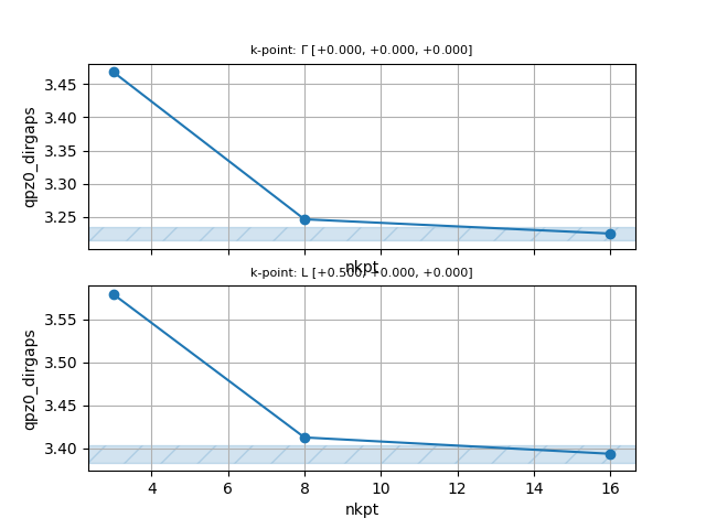
To conclude, our best values for the direct QP gaps are 3.247 eV at the \(\Gamma\)-point and 3.413 eV at the \(L\)-point.
mkdir conv_kmesh
mv conv_kmesh.py conv_kmesh
mv tgwr_4o_* log conv_kmesh
How to compute an interpolated band structure with GWR
In this last part of the tutorial, we discuss how to interpolate the QP corrections along an arbitrary \(\kk\)-path using the star-function method discussed in this section of the EPH introduction. This method is less precise than e.g. the Wannier interpolation, and might be problematic in the presence of band-crossings, but it has the big advantage of being much easier to use and with minimal user intervention.
First of all, we need to compute the QP corrections for all the \(\kk\)-points in the IBZ. This is done in the following input:
# Crystalline silicon
# Calculation of the GW corrections with GWR code and 2x2x2 k-mesh.
# Compute QP corrections for all k-points in the IBZ


# Definition of the k-point grid
# IMPORTANT: GWR requires Gamma-centered k-meshes
ngkpt   2 2 2
#ngkpt   4 4 4
nshiftk 1
shiftk  0.0 0.0 0.0

# Include geometry and pseudos
include "gwr_include.abi"

################################
# Dataset 3: G0W0 with GWR code
################################
optdriver  6                          # Activate GWR code
ecutwfn    10                         # Truncate basis set when computing G.
                                      # This parameter should be subject to convergence studies
gwr_task "G0W0"                       # One-shot calculation
getden_filepath "tgwr_1o_DS1_DEN"     # Density file
getwfk_filepath "tgwr_2o_DS1_WFK"     # WFK file with empty states. Must be consisten with ngkpt, shiftk
#getwfk_filepath "tgwr_2o_DS2_WFK"     # WFK file with empty states. Must be consisten with ngkpt, shiftk

#gwr_ntau   6         # Number of imaginary-time points
gwr_ntau   12         # Number of imaginary-time points
gwr_boxcutmin  1.0  # This should be subject to convergence studies
gwr_sigma_algo 1     # Use supercell for Sigma

nband      250      # Bands to be used in the screening calculation
ecuteps    6        # Cut-off energy of the planewave set to represent the dielectric matrix.
                    # It is important to adjust this parameter.
#ecutsigx  16.0     # Dimension of the G sum in Sigma_x.
                    # ecutsigx = ecut is usually a wise choice
                    # (the dimension in Sigma_c is controlled by ecuteps)
gw_qprange  -4      # Compute the QP corrections for all the k-points in the irreducible zone.
                    # Include all occupied states and -num empty states

# Spectral function (very coarse grid to reduce txt file size)
#nfreqsp3 50
#freqspmax3 5 eV

#%%<BEGIN TEST_INFO>
#%% [setup]
#%% executable = abinit
#%% test_chain = tgwr_1.abi, tgwr_2.abi, tgwr_3.abi, tgwr_4.abi, tgwr_5.abi
#%% need_cpp_vars = HAVE_LINALG_SCALAPACK
#%% exclude_builders = eos_nvhpc_23.9_elpa ,eos_nvhpc_24.9_openmpi, haicgu_*
#%% [files]
#%% files_to_test =
#%%   tgwr_5.abo, tolnlines = 25, tolabs = 1.1e-3, tolrel = 3.0e-3, fld_options = -medium;
#%% [paral_info]
#%% max_nprocs = 12
#%% [extra_info]
#%% authors = M. Giantomassi
#%% keywords = NC, GWR
#%% description =
#%%  Crystalline silicon
#%%  Calculation of the GW corrections with GWR code for all k-points in the IBZ.
#%%<END TEST_INFO>
Note the usage of gw_qprange = -NUM and gwr_sigma_algo 1 to activate
the supercell algorithm for \(\Sigma_\nk\), the most efficient algorithm when all the \(\kk\)-points in \(\Sigma_\nk\) are wanted.
To keep the wall-time at a reasonable level, we use a WFK file with 2x2x2 \(\kk\)-mesh,
but it is clear that a more precise interpolation would require denser \(\kk\)-meshes.
Run the job with:
mpirun -n 1 tgwr_5.abi > tgwr_5.log 2> err &
The output file is reported here for your convenience:
.Version 10.5.8.2 of ABINIT, released Oct 2025.
.(MPI version, prepared for a x86_64_linux_gnu13.2 computer)
.Copyright (C) 1998-2026 ABINIT group .
ABINIT comes with ABSOLUTELY NO WARRANTY.
It is free software, and you are welcome to redistribute it
under certain conditions (GNU General Public License,
see ~abinit/COPYING or http://www.gnu.org/copyleft/gpl.txt).
ABINIT is a project of the Universite Catholique de Louvain,
Corning Inc. and other collaborators, see ~abinit/doc/developers/contributors.txt .
Please read https://docs.abinit.org/theory/acknowledgments for suggested
acknowledgments of the ABINIT effort.
For more information, see https://www.abinit.org .
.Starting date : Sat 20 Dec 2025.
- ( at 17h10 )
- input file -> /home/buildbot/ABINIT3/eos_gnu_13.2_mpich/trunk__codata2022/tests/TestBot_MPI1/tutorial_tgwr_1-tgwr_2-tgwr_3-tgwr_4-tgwr_5/tgwr_5.abi
- output file -> tgwr_5.abo
- root for input files -> tgwr_5i
- root for output files -> tgwr_5o
Symmetries : space group Fd -3 m (#227); Bravais cF (face-center cubic)
================================================================================
Values of the parameters that define the memory need of the present run
intxc = 0 ionmov = 0 iscf = 7 lmnmax = 6
lnmax = 6 mgfft = 30 mpssoang = 3 mqgrid = 3001
natom = 2 nloc_mem = 1 nspden = 1 nspinor = 1
nsppol = 1 nsym = 48 n1xccc = 2501 ntypat = 1
occopt = 1 xclevel = 2
- mband = 250 mffmem = 1 mkmem = 3
mpw = 435 nfft = 27000 nkpt = 3
================================================================================
P This job should need less than 15.687 Mbytes of memory.
Rough estimation (10% accuracy) of disk space for files :
_ WF disk file : 4.980 Mbytes ; DEN or POT disk file : 0.208 Mbytes.
================================================================================
--------------------------------------------------------------------------------
------------- Echo of variables that govern the present computation ------------
--------------------------------------------------------------------------------
-
- outvars: echo of selected default values
- iomode0 = 0 , fftalg0 =512 , wfoptalg0 = 0
-
- outvars: echo of global parameters not present in the input file
- max_nthreads = 0
-
-outvars: echo values of preprocessed input variables --------
acell 1.0260000000E+01 1.0260000000E+01 1.0260000000E+01 Bohr
amu 2.80855000E+01
ecut 1.60000000E+01 Hartree
ecuteps 6.00000000E+00 Hartree
ecutsigx 1.60000000E+01 Hartree
ecutwfn 1.00000000E+01 Hartree
- fftalg 512
gw_qprange -4
istwfk 2 3 7
ixc 11
kpt 0.00000000E+00 0.00000000E+00 0.00000000E+00
5.00000000E-01 0.00000000E+00 0.00000000E+00
5.00000000E-01 5.00000000E-01 0.00000000E+00
kptrlatt 2 0 0 0 2 0 0 0 2
kptrlen 1.45098311E+01
P mkmem 3
natom 2
nband 250
ngfft 30 30 30
nkpt 3
nsym 48
ntypat 1
occ 2.000000 2.000000 2.000000 2.000000 0.000000 0.000000
0.000000 0.000000 0.000000 0.000000 0.000000 0.000000
0.000000 0.000000 0.000000 0.000000 0.000000 0.000000
0.000000 0.000000 0.000000 0.000000 0.000000 0.000000
0.000000 0.000000 0.000000 0.000000 0.000000 0.000000
0.000000 0.000000 0.000000 0.000000 0.000000 0.000000
0.000000 0.000000 0.000000 0.000000 0.000000 0.000000
0.000000 0.000000 0.000000 0.000000 0.000000 0.000000
0.000000 0.000000 0.000000 0.000000 0.000000 0.000000
0.000000 0.000000 0.000000 0.000000 0.000000 0.000000
0.000000 0.000000 0.000000 0.000000 0.000000 0.000000
0.000000 0.000000 0.000000 0.000000 0.000000 0.000000
0.000000 0.000000 0.000000 0.000000 0.000000 0.000000
0.000000 0.000000 0.000000 0.000000 0.000000 0.000000
0.000000 0.000000 0.000000 0.000000 0.000000 0.000000
0.000000 0.000000 0.000000 0.000000 0.000000 0.000000
0.000000 0.000000 0.000000 0.000000 0.000000 0.000000
0.000000 0.000000 0.000000 0.000000 0.000000 0.000000
0.000000 0.000000 0.000000 0.000000 0.000000 0.000000
0.000000 0.000000 0.000000 0.000000 0.000000 0.000000
0.000000 0.000000 0.000000 0.000000 0.000000 0.000000
0.000000 0.000000 0.000000 0.000000 0.000000 0.000000
0.000000 0.000000 0.000000 0.000000 0.000000 0.000000
0.000000 0.000000 0.000000 0.000000 0.000000 0.000000
0.000000 0.000000 0.000000 0.000000 0.000000 0.000000
0.000000 0.000000 0.000000 0.000000 0.000000 0.000000
0.000000 0.000000 0.000000 0.000000 0.000000 0.000000
0.000000 0.000000 0.000000 0.000000 0.000000 0.000000
0.000000 0.000000 0.000000 0.000000 0.000000 0.000000
0.000000 0.000000 0.000000 0.000000 0.000000 0.000000
0.000000 0.000000 0.000000 0.000000 0.000000 0.000000
0.000000 0.000000 0.000000 0.000000 0.000000 0.000000
0.000000 0.000000 0.000000 0.000000 0.000000 0.000000
0.000000 0.000000 0.000000 0.000000 0.000000 0.000000
0.000000 0.000000 0.000000 0.000000 0.000000 0.000000
0.000000 0.000000 0.000000 0.000000 0.000000 0.000000
0.000000 0.000000 0.000000 0.000000 0.000000 0.000000
0.000000 0.000000 0.000000 0.000000 0.000000 0.000000
0.000000 0.000000 0.000000 0.000000 0.000000 0.000000
0.000000 0.000000 0.000000 0.000000 0.000000 0.000000
0.000000 0.000000 0.000000 0.000000 0.000000 0.000000
0.000000 0.000000 0.000000 0.000000
optdriver 6
rprim 0.0000000000E+00 5.0000000000E-01 5.0000000000E-01
5.0000000000E-01 0.0000000000E+00 5.0000000000E-01
5.0000000000E-01 5.0000000000E-01 0.0000000000E+00
spgroup 227
symrel 1 0 0 0 1 0 0 0 1 -1 0 0 0 -1 0 0 0 -1
0 -1 1 0 -1 0 1 -1 0 0 1 -1 0 1 0 -1 1 0
-1 0 0 -1 0 1 -1 1 0 1 0 0 1 0 -1 1 -1 0
0 1 -1 1 0 -1 0 0 -1 0 -1 1 -1 0 1 0 0 1
-1 0 0 -1 1 0 -1 0 1 1 0 0 1 -1 0 1 0 -1
0 -1 1 1 -1 0 0 -1 0 0 1 -1 -1 1 0 0 1 0
1 0 0 0 0 1 0 1 0 -1 0 0 0 0 -1 0 -1 0
0 1 -1 0 0 -1 1 0 -1 0 -1 1 0 0 1 -1 0 1
-1 0 1 -1 1 0 -1 0 0 1 0 -1 1 -1 0 1 0 0
0 -1 0 1 -1 0 0 -1 1 0 1 0 -1 1 0 0 1 -1
1 0 -1 0 0 -1 0 1 -1 -1 0 1 0 0 1 0 -1 1
0 1 0 0 0 1 1 0 0 0 -1 0 0 0 -1 -1 0 0
1 0 -1 0 1 -1 0 0 -1 -1 0 1 0 -1 1 0 0 1
0 -1 0 0 -1 1 1 -1 0 0 1 0 0 1 -1 -1 1 0
-1 0 1 -1 0 0 -1 1 0 1 0 -1 1 0 0 1 -1 0
0 1 0 1 0 0 0 0 1 0 -1 0 -1 0 0 0 0 -1
0 0 -1 0 1 -1 1 0 -1 0 0 1 0 -1 1 -1 0 1
1 -1 0 0 -1 1 0 -1 0 -1 1 0 0 1 -1 0 1 0
0 0 1 1 0 0 0 1 0 0 0 -1 -1 0 0 0 -1 0
-1 1 0 -1 0 0 -1 0 1 1 -1 0 1 0 0 1 0 -1
0 0 1 0 1 0 1 0 0 0 0 -1 0 -1 0 -1 0 0
1 -1 0 0 -1 0 0 -1 1 -1 1 0 0 1 0 0 1 -1
0 0 -1 1 0 -1 0 1 -1 0 0 1 -1 0 1 0 -1 1
-1 1 0 -1 0 1 -1 0 0 1 -1 0 1 0 -1 1 0 0
tnons 0.0000000 0.0000000 0.0000000 0.2500000 0.2500000 0.2500000
0.0000000 0.0000000 0.0000000 0.2500000 0.2500000 0.2500000
0.0000000 0.0000000 0.0000000 0.2500000 0.2500000 0.2500000
0.0000000 0.0000000 0.0000000 0.2500000 0.2500000 0.2500000
0.0000000 0.0000000 0.0000000 0.2500000 0.2500000 0.2500000
0.0000000 0.0000000 0.0000000 0.2500000 0.2500000 0.2500000
0.0000000 0.0000000 0.0000000 0.2500000 0.2500000 0.2500000
0.0000000 0.0000000 0.0000000 0.2500000 0.2500000 0.2500000
0.0000000 0.0000000 0.0000000 0.2500000 0.2500000 0.2500000
0.0000000 0.0000000 0.0000000 0.2500000 0.2500000 0.2500000
0.0000000 0.0000000 0.0000000 0.2500000 0.2500000 0.2500000
0.0000000 0.0000000 0.0000000 0.2500000 0.2500000 0.2500000
0.0000000 0.0000000 0.0000000 0.2500000 0.2500000 0.2500000
0.0000000 0.0000000 0.0000000 0.2500000 0.2500000 0.2500000
0.0000000 0.0000000 0.0000000 0.2500000 0.2500000 0.2500000
0.0000000 0.0000000 0.0000000 0.2500000 0.2500000 0.2500000
0.0000000 0.0000000 0.0000000 0.2500000 0.2500000 0.2500000
0.0000000 0.0000000 0.0000000 0.2500000 0.2500000 0.2500000
0.0000000 0.0000000 0.0000000 0.2500000 0.2500000 0.2500000
0.0000000 0.0000000 0.0000000 0.2500000 0.2500000 0.2500000
0.0000000 0.0000000 0.0000000 0.2500000 0.2500000 0.2500000
0.0000000 0.0000000 0.0000000 0.2500000 0.2500000 0.2500000
0.0000000 0.0000000 0.0000000 0.2500000 0.2500000 0.2500000
0.0000000 0.0000000 0.0000000 0.2500000 0.2500000 0.2500000
typat 1 1
wtk 0.12500 0.50000 0.37500
xangst 0.0000000000E+00 0.0000000000E+00 0.0000000000E+00
1.3573395450E+00 1.3573395450E+00 1.3573395450E+00
xcart 0.0000000000E+00 0.0000000000E+00 0.0000000000E+00
2.5650000000E+00 2.5650000000E+00 2.5650000000E+00
xred 0.0000000000E+00 0.0000000000E+00 0.0000000000E+00
2.5000000000E-01 2.5000000000E-01 2.5000000000E-01
znucl 14.00000
================================================================================
chkinp: Checking input parameters for consistency.
================================================================================
== DATASET 1 ==================================================================
- mpi_nproc: 1, omp_nthreads: -1 (-1 if OMP is not activated)
--- !DatasetInfo
iteration_state: {dtset: 1, }
dimensions: {natom: 2, nkpt: 3, mband: 250, nsppol: 1, nspinor: 1, nspden: 1, mpw: 435, }
cutoff_energies: {ecut: 16.0, pawecutdg: -1.0, }
electrons: {nelect: 8.00000000E+00, charge: 0.00000000E+00, occopt: 1.00000000E+00, tsmear: 1.00000000E-02, }
meta: {optdriver: 6, }
...
mkfilename: getwfk from: tgwr_2o_DS1_WFK
mkfilename: getden from: tgwr_1o_DS1_DEN
Exchange-correlation functional for the present dataset will be:
GGA: Perdew-Burke-Ernzerhof functional - ixc=11
Citation for XC functional:
J.P.Perdew, K.Burke, M.Ernzerhof, PRL 77, 3865 (1996)
.Using double precision arithmetic; gwpc = 8
- Reading GS density from: tgwr_1o_DS1_DEN
--- Pseudopotential description ------------------------------------------------
- pspini: atom type 1 psp file is /home/buildbot/ABINIT3/eos_gnu_13.2_mpich/trunk__codata2022/tests/Pspdir/Psdj_nc_sr_04_pbe_std_psp8/Si.psp8
- pspatm: opening atomic psp file /home/buildbot/ABINIT3/eos_gnu_13.2_mpich/trunk__codata2022/tests/Pspdir/Psdj_nc_sr_04_pbe_std_psp8/Si.psp8
- Si ONCVPSP-3.2.3.1 r_core= 1.60303 1.72197 1.91712
- 14.00000 4.00000 170510 znucl, zion, pspdat
8 11 2 4 600 0.00000 pspcod,pspxc,lmax,lloc,mmax,r2well
5.99000000000000 4.00000000000000 0.00000000000000 rchrg,fchrg,qchrg
nproj 2 2 2
extension_switch 1
pspatm : epsatm= 9.34321699
--- l ekb(1:nproj) -->
0 5.168965 0.829883
1 2.571282 0.578307
2 -2.427311 -0.488097
pspatm: atomic psp has been read and splines computed
1.49491472E+02 ecore*ucvol(ha*bohr**3)
--------------------------------------------------------------------------------
Total charge density [el/Bohr^3]
) Maximum= 8.5569E-02 at reduced coord. 0.1000 0.1000 0.7000
) Minimum= 1.4870E-03 at reduced coord. 0.0000 0.0000 0.0000
Integrated= 8.0000E+00
- Reading GS states from WFK file: tgwr_2o_DS1_WFK
Mapping kBZ --> kIBZ
Legend: bz = TS(ibz) + g0 where isym is the index of the symrec operation S and itim is 1 if TR is used.
BZ IBZ ibz isym itim g0
1 [ 0.0000E+00, 0.0000E+00, 0.0000E+00] [ 0.0000E+00, 0.0000E+00, 0.0000E+00] 1 1 0 [0, 0, 0]
2 [ 5.0000E-01, 0.0000E+00, 0.0000E+00] [ 5.0000E-01, 0.0000E+00, 0.0000E+00] 2 1 0 [0, 0, 0]
3 [ 5.0000E-01, 5.0000E-01, 5.0000E-01] [ 5.0000E-01, 0.0000E+00, 0.0000E+00] 2 5 0 [1, 1, 1]
4 [ 0.0000E+00, 0.0000E+00, 5.0000E-01] [ 5.0000E-01, 0.0000E+00, 0.0000E+00] 2 3 0 [0, 0, 0]
5 [ 0.0000E+00, 5.0000E-01, 0.0000E+00] [ 5.0000E-01, 0.0000E+00, 0.0000E+00] 2 7 0 [0, 0, 0]
6 [ 5.0000E-01, 5.0000E-01, 0.0000E+00] [ 5.0000E-01, 5.0000E-01, 0.0000E+00] 3 1 0 [0, 0, 0]
7 [ 5.0000E-01, 0.0000E+00, 5.0000E-01] [ 5.0000E-01, 5.0000E-01, 0.0000E+00] 3 9 0 [1, 0, 1]
8 [ 0.0000E+00, 5.0000E-01, 5.0000E-01] [ 5.0000E-01, 5.0000E-01, 0.0000E+00] 3 17 0 [0, 0, 0]
Mapping qBZ --> qIBZ
Legend: bz = TS(ibz) + g0 where isym is the index of the symrec operation S and itim is 1 if TR is used.
BZ IBZ ibz isym itim g0
1 [ 0.0000E+00, 0.0000E+00, 0.0000E+00] [ 0.0000E+00, 0.0000E+00, 0.0000E+00] 1 1 0 [0, 0, 0]
2 [ 5.0000E-01, 0.0000E+00, 0.0000E+00] [ 5.0000E-01, 0.0000E+00, 0.0000E+00] 2 1 0 [0, 0, 0]
3 [ 5.0000E-01, 5.0000E-01, 5.0000E-01] [ 5.0000E-01, 0.0000E+00, 0.0000E+00] 2 5 0 [1, 1, 1]
4 [ 0.0000E+00, 0.0000E+00, 5.0000E-01] [ 5.0000E-01, 0.0000E+00, 0.0000E+00] 2 3 0 [0, 0, 0]
5 [ 0.0000E+00, 5.0000E-01, 0.0000E+00] [ 5.0000E-01, 0.0000E+00, 0.0000E+00] 2 7 0 [0, 0, 0]
6 [ 5.0000E-01, 5.0000E-01, 0.0000E+00] [ 5.0000E-01, 5.0000E-01, 0.0000E+00] 3 1 0 [0, 0, 0]
7 [ 5.0000E-01, 0.0000E+00, 5.0000E-01] [ 5.0000E-01, 5.0000E-01, 0.0000E+00] 3 9 0 [1, 0, 1]
8 [ 0.0000E+00, 5.0000E-01, 5.0000E-01] [ 5.0000E-01, 5.0000E-01, 0.0000E+00] 3 17 0 [0, 0, 0]
=== Kohn-Sham gaps and band edges from IBZ mesh ===
Indirect band gap semiconductor
Fundamental gap: 0.707 (eV)
VBM: -0.354 (eV) at k: [ 0.0000E+00, 0.0000E+00, 0.0000E+00]
CBM: 0.354 (eV) at k: [ 5.0000E-01, 5.0000E-01, 0.0000E+00]
Direct gap: 2.556 (eV) at k: [ 0.0000E+00, 0.0000E+00, 0.0000E+00]
- Optimizing MPI grid with mem_per_cpu_mb: 2.048000E+03 [Mb]
- Use `abinit run.abi --mem-per-cpu=4G` to set mem_per_cpu_mb in the submission script
- np_k np_g np_t np_s memb_per_cpu efficiency speedup
- 1 1 1 1 6.11409E+02 1.00000E+00 1.00000E+00
-
- Selected MPI grid:
- np_k np_g np_t np_s memb_per_cpu efficiency speedup
- 1 1 1 1 6.11409E+02 1.00000E+00 1.00000E+00
- Resident memory in Mb for G(g,g',+/-tau) and chi(g,g',tau):
- G_k(g,g,tau): 373.0
- Chi_q(g,g,tau): 19.8
- u_k(g,b): 4.7
- Temporary memory allocated inside the tau loops:
- G_k(r,g): 173.8
- chi_q(r,g): 40.1
P kpt_comm can use shmem: yes
P g_comm can use shmem: yes
P tau_comm can use shmem: yes
P spin_comm can use shmem yes
- FFT uc_batch_size: 1
- FFT sc_batch_size: 1
==== Info on the gwr_t object ====
--- !GWR_params
iteration_state: {dtset: 1, }
gwr_task: G0W0
nband: 250
ntau: 12
ngkpt: [2, 2, 2, ]
ngqpt: [2, 2, 2, ]
chi_algo: supercell
sigma_algo: supercell
nkibz: 3
nqibz: 3
inclvkb: 2
q0: [ 1.00000000E-05, 2.00000000E-05, 3.00000000E-05, ]
gw_icutcoul: 6
green_mpw: 412
tchi_mpw: 190
g_ngfft: [12, 12, 12, 12, 12, 12, ]
gwr_boxcutmin: 1.00000000E+00
P gwr_np_kgts: [1, 1, 1, 1, ]
P np_kibz: [1, 1, 1, ]
P np_qibz: [1, 1, 1, ]
min_transition_energy_eV: 7.07322783E-01
max_transition_energy_eV: 1.90213912E+02
eratio: 2.68920946E+02
ft_max_err_t2w_cos: 1.19214900E-03
ft_max_err_w2t_cos: 3.55934970E-05
ft_max_err_t2w_sin: 2.27327756E-02
cosft_duality_error: 5.10408367E-03
Minimax imaginary tau/omega mesh in a.u.: !Tabular | # tau, weight(tau), omega, weight(omega)
1 3.01845E-02 7.84567E-02 6.37107E-03 1.30197E-02
2 1.68348E-01 2.04750E-01 2.08408E-02 1.65798E-02
3 4.62515E-01 4.00892E-01 4.11428E-02 2.50342E-02
4 1.02120E+00 7.51969E-01 7.35654E-02 4.15594E-02
5 2.06352E+00 1.39686E+00 1.29029E-01 7.25879E-02
6 3.98516E+00 2.55709E+00 2.27719E-01 1.30961E-01
7 7.46798E+00 4.59587E+00 4.08469E-01 2.42767E-01
8 1.36656E+01 8.11373E+00 7.48639E-01 4.62721E-01
9 2.45159E+01 1.41167E+01 1.40860E+00 9.11790E-01
10 4.33066E+01 2.43993E+01 2.74298E+00 1.88995E+00
11 7.59655E+01 4.28466E+01 5.67129E+00 4.41801E+00
12 1.35795E+02 8.33674E+01 1.41554E+01 1.63699E+01
...
Cutting u(g) as ecutwfn: 1.000000E+01 < ecut: 1.600000E+01
Computing chi0 head and wings with inclvkb: 2
Using KS orbitals and KS energies...
Computing diagonal matrix elements of Sigma_x
=== Info on Coulomb term used in Sigma_x ===
cutoff-mode = AUXILIARY_FUNCTION
Using KS orbitals and KS energies...
Building Green's functions from KS orbitals and KS energies...
Building correlated screening Wc(i omega) ...
=== Info on Coulomb term used in epsilon and W ===
cutoff-mode = AUXILIARY_FUNCTION
--- !EMACRO_WITHOUT_LOCAL_FIELDS
iteration_state: {dtset: 1, }
'epsilon_{iw, q -> Gamma}(0,0)': !Tabular |
6.37106624E-03 5.55279726E+01 3.22464522E-17
2.08407959E-02 5.37815014E+01 -1.27102598E-16
4.11427666E-02 4.89350575E+01 -4.56315445E-17
7.35653993E-02 3.89295630E+01 8.44673115E-17
1.29029157E-01 2.46713871E+01 1.01107529E-17
2.27718878E-01 1.21440316E+01 -1.58191073E-17
4.08469196E-01 5.16857531E+00 9.08182639E-19
7.48638937E-01 2.34544068E+00 -1.36840034E-18
1.40860376E+00 1.39397591E+00 3.95508620E-19
2.74297741E+00 1.10584246E+00 -1.44878319E-19
5.67129327E+00 1.02502657E+00 5.38224158E-20
1.41553560E+01 1.00403863E+00 4.76979499E-21
...
--- !EMACRO_WITH_LOCAL_FIELDS
iteration_state: {dtset: 1, }
'epsilon_{iw, q -> Gamma}(0,0)': !Tabular |
6.37106624E-03 2.06795543E-02 0.00000000E+00
2.08407959E-02 2.12825310E-02 0.00000000E+00
4.11427666E-02 2.31803318E-02 0.00000000E+00
7.35653993E-02 2.85859155E-02 0.00000000E+00
1.29029157E-01 4.38160503E-02 0.00000000E+00
2.27718878E-01 8.64291349E-02 0.00000000E+00
4.08469196E-01 1.98525512E-01 0.00000000E+00
7.48638937E-01 4.30694170E-01 0.00000000E+00
1.40860376E+00 7.19057296E-01 0.00000000E+00
2.74297741E+00 9.04569521E-01 0.00000000E+00
5.67129327E+00 9.75607818E-01 0.00000000E+00
1.41553560E+01 9.95978327E-01 0.00000000E+00
...
Computing diagonal matrix elements of Sigma_c
=== Info on Coulomb term used in Sigma_c ===
cutoff-mode = AUXILIARY_FUNCTION
================================================================================
QP results (energies in eV)
Notations:
E0: Kohn-Sham energy
<VxcDFT>: Matrix elements of Vxc[n_val] without non-linear core correction (if any)
SigX: Matrix elements of Sigma_x
SigC(E0): Matrix elements of Sigma_c at E0
Z: Renormalization factor
E-E0: Difference between the QP and the KS energy.
E-Eprev: Difference between QP energy at iteration i and i-1
E: Quasi-particle energy
Occ(E): Occupancy of QP state
--- !GWR_SelfEnergy_ee
iteration_state: {dtset: 1, }
kpoint : [ 0.000, 0.000, 0.000, ]
spin : 1
gwr_scf_iteration: 1
gwr_task : G0W0
QP_VBM_band: 2
QP_CBM_band: 5
KS_gap : 2.556
QP_gap : 3.449
Delta_QP_KS: 0.893
data: !Tabular |
Band E0 <VxcDFT> SigX SigC(E0) Z E-E0 E-Eprev E Occ(E)
1 -12.323 -10.470 -16.449 5.548 0.716 -0.049 -0.049 -12.373 2.000
2 -0.354 -11.319 -13.616 1.514 0.777 -0.459 -0.459 -0.813 2.000
3 -0.354 -11.319 -13.616 1.514 0.777 -0.460 -0.460 -0.813 2.000
4 -0.354 -11.319 -13.616 1.514 0.777 -0.459 -0.459 -0.813 2.000
5 2.202 -10.034 -4.915 -4.753 0.778 0.434 0.434 2.636 0.000
6 2.202 -10.034 -4.915 -4.753 0.778 0.434 0.434 2.636 0.000
7 2.202 -10.034 -4.915 -4.753 0.778 0.434 0.434 2.636 0.000
8 2.996 -10.917 -5.006 -5.493 0.769 0.470 0.470 3.466 0.000
...
--- !GWR_SelfEnergy_ee
iteration_state: {dtset: 1, }
kpoint : [ 0.500, 0.000, 0.000, ]
spin : 1
gwr_scf_iteration: 1
gwr_task : G0W0
QP_VBM_band: 3
QP_CBM_band: 5
KS_gap : 2.733
QP_gap : 3.578
Delta_QP_KS: 0.845
data: !Tabular |
Band E0 <VxcDFT> SigX SigC(E0) Z E-E0 E-Eprev E Occ(E)
1 -9.991 -10.853 -15.973 4.636 0.732 -0.147 -0.147 -10.138 2.000
2 -7.331 -10.209 -13.774 3.120 0.761 -0.171 -0.171 -7.502 2.000
3 -1.556 -11.058 -13.442 1.686 0.774 -0.391 -0.391 -1.947 2.000
4 -1.556 -11.058 -13.442 1.686 0.774 -0.392 -0.392 -1.947 2.000
5 1.177 -10.088 -5.037 -4.663 0.786 0.454 0.454 1.631 0.000
6 2.983 -9.664 -4.428 -4.837 0.784 0.461 0.461 3.445 0.000
7 2.983 -9.664 -4.428 -4.838 0.784 0.461 0.461 3.444 0.000
8 7.378 -7.761 -2.017 -5.677 0.789 0.192 0.192 7.571 0.000
...
--- !GWR_SelfEnergy_ee
iteration_state: {dtset: 1, }
kpoint : [ 0.500, 0.500, 0.000, ]
spin : 1
gwr_scf_iteration: 1
gwr_task : G0W0
QP_VBM_band: 4
QP_CBM_band: 5
KS_gap : 3.565
QP_gap : 4.326
Delta_QP_KS: 0.761
data: !Tabular |
Band E0 <VxcDFT> SigX SigC(E0) Z E-E0 E-Eprev E Occ(E)
1 -8.178 -10.852 -15.143 3.805 0.745 -0.183 -0.183 -8.361 2.000
2 -8.178 -10.852 -15.143 3.805 0.745 -0.183 -0.183 -8.361 2.000
3 -3.211 -10.592 -13.169 1.991 0.770 -0.302 -0.302 -3.513 2.000
4 -3.211 -10.592 -13.169 1.991 0.770 -0.302 -0.302 -3.513 2.000
5 0.354 -8.989 -4.197 -4.403 0.800 0.459 0.459 0.813 0.000
6 0.354 -8.989 -4.197 -4.403 0.800 0.459 0.459 0.813 0.000
7 9.744 -10.558 -3.773 -6.677 0.756 0.198 0.198 9.942 0.000
8 9.744 -10.558 -3.773 -6.678 0.756 0.197 0.197 9.941 0.000
...
=== Kohn-Sham gaps and band edges from IBZ mesh ===
Indirect band gap semiconductor
Fundamental gap: 0.707 (eV)
VBM: -0.354 (eV) at k: [ 0.0000E+00, 0.0000E+00, 0.0000E+00]
CBM: 0.354 (eV) at k: [ 5.0000E-01, 5.0000E-01, 0.0000E+00]
Direct gap: 2.556 (eV) at k: [ 0.0000E+00, 0.0000E+00, 0.0000E+00]
=== QP gaps and band edges taking into account Sigma_nk corrections for 3 k-points ===
Indirect band gap semiconductor
Fundamental gap: 1.626 (eV)
VBM: -0.813 (eV) at k: [ 0.0000E+00, 0.0000E+00, 0.0000E+00]
CBM: 0.813 (eV) at k: [ 5.0000E-01, 5.0000E-01, 0.0000E+00]
Direct gap: 3.449 (eV) at k: [ 0.0000E+00, 0.0000E+00, 0.0000E+00]
== END DATASET(S) ==============================================================
================================================================================
-outvars: echo values of variables after computation --------
acell 1.0260000000E+01 1.0260000000E+01 1.0260000000E+01 Bohr
amu 2.80855000E+01
ecut 1.60000000E+01 Hartree
ecuteps 6.00000000E+00 Hartree
ecutsigx 1.60000000E+01 Hartree
ecutwfn 1.00000000E+01 Hartree
etotal 0.0000000000E+00
fcart 0.0000000000E+00 0.0000000000E+00 0.0000000000E+00
0.0000000000E+00 0.0000000000E+00 0.0000000000E+00
- fftalg 512
gw_qprange -4
istwfk 2 3 7
ixc 11
kpt 0.00000000E+00 0.00000000E+00 0.00000000E+00
5.00000000E-01 0.00000000E+00 0.00000000E+00
5.00000000E-01 5.00000000E-01 0.00000000E+00
kptrlatt 2 0 0 0 2 0 0 0 2
kptrlen 1.45098311E+01
P mkmem 3
natom 2
nband 250
ngfft 30 30 30
nkpt 3
nsym 48
ntypat 1
occ 2.000000 2.000000 2.000000 2.000000 0.000000 0.000000
0.000000 0.000000 0.000000 0.000000 0.000000 0.000000
0.000000 0.000000 0.000000 0.000000 0.000000 0.000000
0.000000 0.000000 0.000000 0.000000 0.000000 0.000000
0.000000 0.000000 0.000000 0.000000 0.000000 0.000000
0.000000 0.000000 0.000000 0.000000 0.000000 0.000000
0.000000 0.000000 0.000000 0.000000 0.000000 0.000000
0.000000 0.000000 0.000000 0.000000 0.000000 0.000000
0.000000 0.000000 0.000000 0.000000 0.000000 0.000000
0.000000 0.000000 0.000000 0.000000 0.000000 0.000000
0.000000 0.000000 0.000000 0.000000 0.000000 0.000000
0.000000 0.000000 0.000000 0.000000 0.000000 0.000000
0.000000 0.000000 0.000000 0.000000 0.000000 0.000000
0.000000 0.000000 0.000000 0.000000 0.000000 0.000000
0.000000 0.000000 0.000000 0.000000 0.000000 0.000000
0.000000 0.000000 0.000000 0.000000 0.000000 0.000000
0.000000 0.000000 0.000000 0.000000 0.000000 0.000000
0.000000 0.000000 0.000000 0.000000 0.000000 0.000000
0.000000 0.000000 0.000000 0.000000 0.000000 0.000000
0.000000 0.000000 0.000000 0.000000 0.000000 0.000000
0.000000 0.000000 0.000000 0.000000 0.000000 0.000000
0.000000 0.000000 0.000000 0.000000 0.000000 0.000000
0.000000 0.000000 0.000000 0.000000 0.000000 0.000000
0.000000 0.000000 0.000000 0.000000 0.000000 0.000000
0.000000 0.000000 0.000000 0.000000 0.000000 0.000000
0.000000 0.000000 0.000000 0.000000 0.000000 0.000000
0.000000 0.000000 0.000000 0.000000 0.000000 0.000000
0.000000 0.000000 0.000000 0.000000 0.000000 0.000000
0.000000 0.000000 0.000000 0.000000 0.000000 0.000000
0.000000 0.000000 0.000000 0.000000 0.000000 0.000000
0.000000 0.000000 0.000000 0.000000 0.000000 0.000000
0.000000 0.000000 0.000000 0.000000 0.000000 0.000000
0.000000 0.000000 0.000000 0.000000 0.000000 0.000000
0.000000 0.000000 0.000000 0.000000 0.000000 0.000000
0.000000 0.000000 0.000000 0.000000 0.000000 0.000000
0.000000 0.000000 0.000000 0.000000 0.000000 0.000000
0.000000 0.000000 0.000000 0.000000 0.000000 0.000000
0.000000 0.000000 0.000000 0.000000 0.000000 0.000000
0.000000 0.000000 0.000000 0.000000 0.000000 0.000000
0.000000 0.000000 0.000000 0.000000 0.000000 0.000000
0.000000 0.000000 0.000000 0.000000 0.000000 0.000000
0.000000 0.000000 0.000000 0.000000
optdriver 6
rprim 0.0000000000E+00 5.0000000000E-01 5.0000000000E-01
5.0000000000E-01 0.0000000000E+00 5.0000000000E-01
5.0000000000E-01 5.0000000000E-01 0.0000000000E+00
spgroup 227
strten 0.0000000000E+00 0.0000000000E+00 0.0000000000E+00
0.0000000000E+00 0.0000000000E+00 0.0000000000E+00
symrel 1 0 0 0 1 0 0 0 1 -1 0 0 0 -1 0 0 0 -1
0 -1 1 0 -1 0 1 -1 0 0 1 -1 0 1 0 -1 1 0
-1 0 0 -1 0 1 -1 1 0 1 0 0 1 0 -1 1 -1 0
0 1 -1 1 0 -1 0 0 -1 0 -1 1 -1 0 1 0 0 1
-1 0 0 -1 1 0 -1 0 1 1 0 0 1 -1 0 1 0 -1
0 -1 1 1 -1 0 0 -1 0 0 1 -1 -1 1 0 0 1 0
1 0 0 0 0 1 0 1 0 -1 0 0 0 0 -1 0 -1 0
0 1 -1 0 0 -1 1 0 -1 0 -1 1 0 0 1 -1 0 1
-1 0 1 -1 1 0 -1 0 0 1 0 -1 1 -1 0 1 0 0
0 -1 0 1 -1 0 0 -1 1 0 1 0 -1 1 0 0 1 -1
1 0 -1 0 0 -1 0 1 -1 -1 0 1 0 0 1 0 -1 1
0 1 0 0 0 1 1 0 0 0 -1 0 0 0 -1 -1 0 0
1 0 -1 0 1 -1 0 0 -1 -1 0 1 0 -1 1 0 0 1
0 -1 0 0 -1 1 1 -1 0 0 1 0 0 1 -1 -1 1 0
-1 0 1 -1 0 0 -1 1 0 1 0 -1 1 0 0 1 -1 0
0 1 0 1 0 0 0 0 1 0 -1 0 -1 0 0 0 0 -1
0 0 -1 0 1 -1 1 0 -1 0 0 1 0 -1 1 -1 0 1
1 -1 0 0 -1 1 0 -1 0 -1 1 0 0 1 -1 0 1 0
0 0 1 1 0 0 0 1 0 0 0 -1 -1 0 0 0 -1 0
-1 1 0 -1 0 0 -1 0 1 1 -1 0 1 0 0 1 0 -1
0 0 1 0 1 0 1 0 0 0 0 -1 0 -1 0 -1 0 0
1 -1 0 0 -1 0 0 -1 1 -1 1 0 0 1 0 0 1 -1
0 0 -1 1 0 -1 0 1 -1 0 0 1 -1 0 1 0 -1 1
-1 1 0 -1 0 1 -1 0 0 1 -1 0 1 0 -1 1 0 0
tnons 0.0000000 0.0000000 0.0000000 0.2500000 0.2500000 0.2500000
0.0000000 0.0000000 0.0000000 0.2500000 0.2500000 0.2500000
0.0000000 0.0000000 0.0000000 0.2500000 0.2500000 0.2500000
0.0000000 0.0000000 0.0000000 0.2500000 0.2500000 0.2500000
0.0000000 0.0000000 0.0000000 0.2500000 0.2500000 0.2500000
0.0000000 0.0000000 0.0000000 0.2500000 0.2500000 0.2500000
0.0000000 0.0000000 0.0000000 0.2500000 0.2500000 0.2500000
0.0000000 0.0000000 0.0000000 0.2500000 0.2500000 0.2500000
0.0000000 0.0000000 0.0000000 0.2500000 0.2500000 0.2500000
0.0000000 0.0000000 0.0000000 0.2500000 0.2500000 0.2500000
0.0000000 0.0000000 0.0000000 0.2500000 0.2500000 0.2500000
0.0000000 0.0000000 0.0000000 0.2500000 0.2500000 0.2500000
0.0000000 0.0000000 0.0000000 0.2500000 0.2500000 0.2500000
0.0000000 0.0000000 0.0000000 0.2500000 0.2500000 0.2500000
0.0000000 0.0000000 0.0000000 0.2500000 0.2500000 0.2500000
0.0000000 0.0000000 0.0000000 0.2500000 0.2500000 0.2500000
0.0000000 0.0000000 0.0000000 0.2500000 0.2500000 0.2500000
0.0000000 0.0000000 0.0000000 0.2500000 0.2500000 0.2500000
0.0000000 0.0000000 0.0000000 0.2500000 0.2500000 0.2500000
0.0000000 0.0000000 0.0000000 0.2500000 0.2500000 0.2500000
0.0000000 0.0000000 0.0000000 0.2500000 0.2500000 0.2500000
0.0000000 0.0000000 0.0000000 0.2500000 0.2500000 0.2500000
0.0000000 0.0000000 0.0000000 0.2500000 0.2500000 0.2500000
0.0000000 0.0000000 0.0000000 0.2500000 0.2500000 0.2500000
typat 1 1
wtk 0.12500 0.50000 0.37500
xangst 0.0000000000E+00 0.0000000000E+00 0.0000000000E+00
1.3573395450E+00 1.3573395450E+00 1.3573395450E+00
xcart 0.0000000000E+00 0.0000000000E+00 0.0000000000E+00
2.5650000000E+00 2.5650000000E+00 2.5650000000E+00
xred 0.0000000000E+00 0.0000000000E+00 0.0000000000E+00
2.5000000000E-01 2.5000000000E-01 2.5000000000E-01
znucl 14.00000
================================================================================
- Timing analysis has been suppressed with timopt=0
================================================================================
Suggested references for the acknowledgment of ABINIT usage.
The users of ABINIT have little formal obligations with respect to the ABINIT group
(those specified in the GNU General Public License, http://www.gnu.org/copyleft/gpl.txt).
However, it is common practice in the scientific literature,
to acknowledge the efforts of people that have made the research possible.
In this spirit, please find below suggested citations of work written by ABINIT developers,
corresponding to implementations inside of ABINIT that you have used in the present run.
Note also that it will be of great value to readers of publications presenting these results,
to read papers enabling them to understand the theoretical formalism and details
of the ABINIT implementation.
For information on why they are suggested, see also https://docs.abinit.org/theory/acknowledgments.
-
- [1] The Abinit project: Impact, environment and recent developments.
- Computer Phys. Comm. 248, 107042 (2020).
- X.Gonze, B. Amadon, G. Antonius, F.Arnardi, L.Baguet, J.-M.Beuken,
- J.Bieder, F.Bottin, J.Bouchet, E.Bousquet, N.Brouwer, F.Bruneval,
- G.Brunin, T.Cavignac, J.-B. Charraud, Wei Chen, M.Cote, S.Cottenier,
- J.Denier, G.Geneste, Ph.Ghosez, M.Giantomassi, Y.Gillet, O.Gingras,
- D.R.Hamann, G.Hautier, Xu He, N.Helbig, N.Holzwarth, Y.Jia, F.Jollet,
- W.Lafargue-Dit-Hauret, K.Lejaeghere, M.A.L.Marques, A.Martin, C.Martins,
- H.P.C. Miranda, F.Naccarato, K. Persson, G.Petretto, V.Planes, Y.Pouillon,
- S.Prokhorenko, F.Ricci, G.-M.Rignanese, A.H.Romero, M.M.Schmitt, M.Torrent,
- M.J.van Setten, B.Van Troeye, M.J.Verstraete, G.Zerah and J.W.Zwanzig
- Comment: the fifth generic paper describing the ABINIT project.
- Note that a version of this paper, that is not formatted for Computer Phys. Comm.
- is available at https://www.abinit.org/sites/default/files/ABINIT20.pdf .
- The licence allows the authors to put it on the Web.
- DOI and bibtex: see https://docs.abinit.org/theory/bibliography/#gonze2020
-
- [2] Optimized norm-conserving Vanderbilt pseudopotentials.
- D.R. Hamann, Phys. Rev. B 88, 085117 (2013).
- Comment: Some pseudopotential generated using the ONCVPSP code were used.
- DOI and bibtex: see https://docs.abinit.org/theory/bibliography/#hamann2013
-
- [3] ABINIT: Overview, and focus on selected capabilities
- J. Chem. Phys. 152, 124102 (2020).
- A. Romero, D.C. Allan, B. Amadon, G. Antonius, T. Applencourt, L.Baguet,
- J.Bieder, F.Bottin, J.Bouchet, E.Bousquet, F.Bruneval,
- G.Brunin, D.Caliste, M.Cote,
- J.Denier, C. Dreyer, Ph.Ghosez, M.Giantomassi, Y.Gillet, O.Gingras,
- D.R.Hamann, G.Hautier, F.Jollet, G. Jomard,
- A.Martin,
- H.P.C. Miranda, F.Naccarato, G.Petretto, N.A. Pike, V.Planes,
- S.Prokhorenko, T. Rangel, F.Ricci, G.-M.Rignanese, M.Royo, M.Stengel, M.Torrent,
- M.J.van Setten, B.Van Troeye, M.J.Verstraete, J.Wiktor, J.W.Zwanziger, and X.Gonze.
- Comment: a global overview of ABINIT, with focus on selected capabilities .
- Note that a version of this paper, that is not formatted for J. Chem. Phys
- is available at https://www.abinit.org/sites/default/files/ABINIT20_JPC.pdf .
- The licence allows the authors to put it on the Web.
- DOI and bibtex: see https://docs.abinit.org/theory/bibliography/#romero2020
-
- [4] Recent developments in the ABINIT software package.
- Computer Phys. Comm. 205, 106 (2016).
- X.Gonze, F.Jollet, F.Abreu Araujo, D.Adams, B.Amadon, T.Applencourt,
- C.Audouze, J.-M.Beuken, J.Bieder, A.Bokhanchuk, E.Bousquet, F.Bruneval
- D.Caliste, M.Cote, F.Dahm, F.Da Pieve, M.Delaveau, M.Di Gennaro,
- B.Dorado, C.Espejo, G.Geneste, L.Genovese, A.Gerossier, M.Giantomassi,
- Y.Gillet, D.R.Hamann, L.He, G.Jomard, J.Laflamme Janssen, S.Le Roux,
- A.Levitt, A.Lherbier, F.Liu, I.Lukacevic, A.Martin, C.Martins,
- M.J.T.Oliveira, S.Ponce, Y.Pouillon, T.Rangel, G.-M.Rignanese,
- A.H.Romero, B.Rousseau, O.Rubel, A.A.Shukri, M.Stankovski, M.Torrent,
- M.J.Van Setten, B.Van Troeye, M.J.Verstraete, D.Waroquier, J.Wiktor,
- B.Xu, A.Zhou, J.W.Zwanziger.
- Comment: the fourth generic paper describing the ABINIT project.
- Note that a version of this paper, that is not formatted for Computer Phys. Comm.
- is available at https://www.abinit.org/sites/default/files/ABINIT16.pdf .
- The licence allows the authors to put it on the Web.
- DOI and bibtex: see https://docs.abinit.org/theory/bibliography/#gonze2016
-
- And optionally:
-
- [5] ABINIT: First-principles approach of materials and nanosystem properties.
- Computer Phys. Comm. 180, 2582-2615 (2009).
- X. Gonze, B. Amadon, P.-M. Anglade, J.-M. Beuken, F. Bottin, P. Boulanger, F. Bruneval,
- D. Caliste, R. Caracas, M. Cote, T. Deutsch, L. Genovese, Ph. Ghosez, M. Giantomassi
- S. Goedecker, D.R. Hamann, P. Hermet, F. Jollet, G. Jomard, S. Leroux, M. Mancini, S. Mazevet,
- M.J.T. Oliveira, G. Onida, Y. Pouillon, T. Rangel, G.-M. Rignanese, D. Sangalli, R. Shaltaf,
- M. Torrent, M.J. Verstraete, G. Zerah, J.W. Zwanziger
- Comment: the third generic paper describing the ABINIT project.
- Note that a version of this paper, that is not formatted for Computer Phys. Comm.
- is available at https://www.abinit.org/sites/default/files/ABINIT_CPC_v10.pdf .
- The licence allows the authors to put it on the Web.
- DOI and bibtex: see https://docs.abinit.org/theory/bibliography/#gonze2009
-
- Proc. 0 individual time (sec): cpu= 88.1 wall= 88.2
================================================================================
Calculation completed.
.Delivered 1 WARNINGs and 6 COMMENTs to log file.
+Overall time at end (sec) : cpu= 88.1 wall= 88.2
Now use the following AbiPy script to read the GWR results and interpolate the QP corrections.
In this case, we pass the KS band structure stored in tgwr_1o_DS2_GSR.nc.
This is the recommended approach as AbiPy will interpolate the QP corrections rather that the QP energies.
The interpolated QP corrections will then be added to the KS energies
thus improving the stability of the interpolation method as QP corrections
are usually smoother than QP energies.
#!/usr/bin/env python
from abipy.electrons.gwr import GwrFile

gwr = GwrFile("tgwr_5o_GWR.nc")
r = gwr.interpolate(ks_ebands_kpath="tgwr_1o_DS2_GSR.nc")

from abipy.electrons.ebands import ElectronBandsPlotter
plotter = ElectronBandsPlotter()
plotter.add_ebands("KS", r.ks_ebands_kpath)
plotter.add_ebands("$G_0W_0$", r.qp_ebands_kpath)

#r.qp_ebands_kpath.plot(with_gaps=True)

plotter.combiplot(savefig="gw_vs_ks_bands.png")
#plotter.gridplot()
Save the script in a file, let’s say plot_qpbands.py, in the same
directory where we have launched the calculation, make the file executable and run it.
You should get the following figures: