First tutorial on DFPT

Dynamical and dielectric properties of AlAs

In this tutorial you will learn how to get the following physical properties (of an insulator) from density-functional perturbation theory (DFPT):

• the phonon frequencies and eigenvectors at $\Gamma$
• the dielectric constant
• the Born effective charges
• the LO-TO splitting
• the phonon frequencies and eigenvectors at other q-points in the Brillouin Zone

In order to learn the use of the associated codes mrgddb and anaddb, to produce phonon band structures and the associated thermodynamical properties, please consult the second tutorial on DFPT.

It is strongly recommended to discover this tutorial simultaneously with the DFPT (respfn) user guide. You might start by reading sections 0 and the first paragraph of section 1 of this user guide.

A basic introduction to the theory is given in [gonze2005]. You might also benefit from reading the longer review [baroni2001]. Further details are in [Gonze1997] and [Gonze1997a].

This tutorial should take about 2 hours.

Note

Supposing you made your own installation of ABINIT, the input files to run the examples are in the ~abinit/tests/ directory where ~abinit is the absolute path of the abinit top-level directory. If you have NOT made your own install, ask your system administrator where to find the package, especially the executable and test files.

In case you work on your own PC or workstation, to make things easier, we suggest you define some handy environment variables by executing the following lines in the terminal:

export ABI_HOME=Replace_with_absolute_path_to_abinit_top_level_dir # Change this line
export PATH=$ABI_HOME/src/98_main/:$PATH      # Do not change this line: path to executable
export ABI_TESTS=$ABI_HOME/tests/             # Do not change this line: path to tests dir
export ABI_PSPDIR=$ABI_TESTS/Psps_for_tests/  # Do not change this line: path to pseudos dir

Examples in this tutorial use these shell variables: copy and paste the code snippets into the terminal (remember to set ABI_HOME first!) or, alternatively, source the set_abienv.sh script located in the ~abinit directory:

source ~abinit/set_abienv.sh

The ‘export PATH’ line adds the directory containing the executables to your PATH so that you can invoke the code by simply typing abinit in the terminal instead of providing the absolute path.

To execute the tutorials, create a working directory (Work*) and copy there the input files of the lesson.

Most of the tutorials do not rely on parallelism (except specific tutorials on parallelism). However you can run most of the tutorial examples in parallel with MPI, see the topic on parallelism.

1 The ground-state geometry of AlAs

Before beginning, you might consider to work in a different subdirectory as for the other tutorials. Why not create Work_rf1 in $ABI_TESTS/tutorespfn/Input?

cd $ABI_TESTS/tutorespfn/Input
mkdir Work_rf1
cd Work_rf1
cp ../trf1_1.abi .

Important

The reference directory that contains the example files for the tutorial is no more $ABI_TESTS/tutorial(as for the basic tutorials and the specialized, non-DFPT ones), but $ABI_TESTS/tutorespfn. This will be the case for all the DFPT based part of the tutorial.

Note that two pseudopotentials are mentioned in the input file: one for the Aluminum atom, and one for the Arsenic atom. The first listed in trf1_1.abi (for Al) will define the first type of atom of the input file (see input variables typat and ntypat) and the second (for As) will define the second type of atom. It might be the first time that you encounter this situation (more than one type of atoms) in the tutorials, at variance with the first four basic tutorials.

Warning

To access the pseudopotential, the input file expect you to define the variable ABI_PSPDIR in your environment.

You can copy the file $ABI_TESTS/tutorespfn/Input/trf1_1.abi in Work_rf1. This is your input file. You should read it carefully.

View tests/tutorespfn/Input/trf1_1.abi

It drives a single self-consistent calculation of the total energy of AlAs to generate the corresponding self-consistent charge density and wavefunctions, that will be used for the DFPT calculations.

Note that the value of tolvrs is rather stringent. This is because the wavefunctions determined by the present run will be used later as starting point of the DFPT calculation. The number of steps, nstep, in this example file has been set to 25. You should always choose a large enough value of nstep to reach your tolvrs target.

Danger

Do not follow blindly all examples of the tutorials: always check the convergence of your calculations while in production!

You will work at fixed ecut (3Ha) and k-point grid, defined by kptrlatt (the 8x8x8 Monkhorst-Pack grid). In real life you should do a convergence test with respect to both parameters. We postpone the discussion of the accuracy of these choices and the choice of pseudopotential to the end of the fifth section of this tutorial. They give acceptable but not very accurate results such that the running time is reasonable for a tutorial.

You should make the run (a few seconds):

abinit trf1_1.abi > log 2> err

The resulting main output file, trf1_1.abo, should be similar to the one below:

View tests/tutorespfn/Refs/trf1_1.abo

This output file is not very long, so you can quickly read it entirely. Note that one obtains the following value for the energy, in the final echo section:

 etotal   -9.7626837450E+00
 etotal   -9.7658722915E+00

However, we will rely later, for the purpose of doing finite differences, on a more accurate (more digits) value of this total energy, that can be found about a dozen of lines before this final echo:

total_energy        : -9.76587229147669E+00

The output file also mentions that the forces on both atoms vanish.

The run that you just made will be considered as defining a ground-state configuration, on top of which responses to perturbations will be computed. The main output of this ground-state run is the wavefunction file trf1_1o_WFK, that you can already rename as trf1_2i_WFK to use it as input wave function for the next runs.

2 Frozen-phonon calculation of a second derivative of the total energy

We will now compute the second derivative of the total energy with respect to an atomic displacement by different means. For that purpose, you must first read sections 0 and the first paragraph of section 1 of the respfn help file (an auxiliary help file, that deals specifically with the DFPT(respfn) features). We will explain later, in more detail, the signification of the different input parameters introduced in section 1 of the respfn help file.

For the time being, in order to be able to perform a direct comparison with the result of a DFPT calculation, we choose as a perturbation the displacement of the Al atom along the first axis of the reduced coordinates.

You can copy the file $ABI_TESTS/tutorespfn/Input/trf1_2.abi in Work_rf1. This is your input file. You should open it and briefly look at the two changes with respect to trf1_1.abi: the change of xred, and the reading of the wavefunction file, using the irdwfk input variable.

Warning

You need to copy trf1_1o_WFK to trf1_2i_WFK so Abinit can find the wavefunction during the calculation.

Then, you can make the run, following the same command as before, with a different files file, referring to trf1_2.abi. The symmetry is lowered with respect to the ground-state geometry, so that the number of k-points increases a lot, and of course, the CPU time.

View tests/tutorespfn/Input/trf1_2.abi View tests/tutorespfn/Refs/trf1_2.abo

From this run, it is possible to get the values of the total energy, and the value of the gradient of the total energy (dE) with respect to change of reduced coordinate (dt):

 rms dE/dt=  3.5517E-03; max dE/dt=  5.0080E-03; dE/dt below (all hartree)
    1       0.005007986445      0.002526333145      0.002526333145
    2      -0.005007927934     -0.002526305645     -0.002526305645
        ...
total_energy        : -9.76586978750721E+00

The change of reduced coordinate (xred) of the Al atom along the first axis was rather small (1/1000 = 0.001), and we can make an estimate of the second derivative of the total energy with respect to the reduced coordinate thanks to finite-difference formulas.

We start first from the total-energy difference. The total energy is symmetric with respect to that perturbation, so that it has no linear term. The difference between the ground-state value (-9.76587229147669E+00 Hartree) of the previous run, and the perturbed value (-9.76586978750721E+00 Hartree) of the present one, is thus one half of the square of the coordinate change (0.001) times the second derivative of total energy (2DTE). From these number, the 2DTE is 5.00793896 Hartree.

Alternatively, we can start from the reduced gradients. The value of the reduced gradient with respect to a displacement of the Al atom along the first reduced axis is 0.005007986445 Ha. At first order, this quantity is the product of the 2DTE by the reduced coordinate difference. The estimate of the 2DTE is thus 5.007986445 Ha. The agreement with the other estimate is rather good (4.10^-5 Hartree).

However, it is possible to do much better, thanks to the use of a higher-order finite-difference formula. For this purpose, one can perform another calculation, in which the change of reduced coordinate along the first axis is 0.002, instead of 0.001. The doubling of the perturbation allows for a rather simple higher-order estimation, as we will see later. The results of this calculation are as follows:

 rms dE/dt=  7.1249E-03; max dE/dt=  1.0016E-02; dE/dt below (all hartree)
1       0.010016404892      0.005097557910      0.005097557910
    2      -0.010016285027     -0.005097505086     -0.005097505086
    ...
 total_energy        : -9.76586227537498E+00

From these data, taking into account that the perturbation was twice stronger, the same procedure as above leads to the values 5.008050855 Hartree (from finite difference of energy) and 5.008202446 Hartree (from finite difference of forces, the value 0.010016404892 has to be multiplied by 1000/2).

The combination of these data with the previous estimate can be done thanks to an higher-order finite-difference formula, in which the difference of estimations (the largest perturbation minus the smallest one) is divided by three, and then subtracted from the smallest estimation.

As far as the total-energy estimation is concerned, the difference is 0.000111895 Ha, which divided by three and subtracted from 5.00793896 Hartree, gives 5.007901661 Hartree. The same higher-order procedure for force estimates gives 5.00791444 Hartree. So, the agreement between total-energy estimate and force estimate of the 2DTE can be observed up to the 6^th digit, inclusive.

Before comparing this result with the 2DTE directly computed from the DFPT capabilities of ABINIT, a last comment is in order. One can observe that the action-reaction law is fulfilled only approximately by the system. Indeed, the force created on the second atom, should be exactly equal in magnitude to the force on the first atom. The values of dE/dt, mentioned above show a small, but non-negligible difference between the two atoms. As an example, for the doubled perturbation, there is a difference in the absolute values of the first component of the reduced force, 0.010016404892 and -0.010016285027.

Actually, the forces should cancel each other exactly if the translation symmetry is perfect. This is not the case, but the breaking of this symmetry can be shown to arise only from the presence of the exchange-correlation grid of points. This grid does not move when atoms are displaced, and so there is a very small variation of the total energy when the system is moved as a whole. It is easy to restore the action-reaction law, by subtracting from every force component the mean of the forces on all atoms. This is actually done when the gradient with respect to reduced coordinates are transformed into forces, and specified in cartesian coordinates, as can be seen in the output file for the small displacement:

 cartesian forces (hartree/bohr) at end:
1     -0.00001684430130    -0.00094404759278    -0.00094404759278
    2      0.00001684430130     0.00094404759278     0.00094404759278

This effect will be seen also at the level of 2DTE. The so-called acoustic sum rule, which imposes that the frequency of three modes (called acoustic modes) tends to zero with vanishing wavevector, will also be slightly broken. In this case, it will also be rather easy to reimpose the acoustic sum rule. In any case, taking a finer XC grid will allow one to reduce this effect.

3 DFPT calculation of a second derivative of the total energy

We now compute the second derivative of the total energy with respect to the same atomic displacement through the DFPT capabilities of ABINIT.

You can copy the file $ABI_TESTS/tutorespfn/Input/trf1_3.abi in Work_rf1. This is your input file. You should examine it. The changes with respect to trf1_1.abi are all gathered in the first part of this file, before

#######################################################################
#Common input variables

Accordingly, you should get familiarized with the new input variables: rfphon, rfatpol, rfdir. Then, pay attention to the special use of the kptopt input variable. It will be explained in more detail later.

Warning

You need to copy trf1_1o_WFK to trf1_3i_WFK so Abinit can find the wavefunction during the calculation.

View tests/tutorespfn/Input/trf1_3.abi

When you have understood the purpose of the input variable values specified before the “Common input variables” section, you can make the code run, as usual.

Then, we need to analyze the different output files. For that purpose, you should read the content of the section 6 of the respfn help file. Read it quickly, as we will come back to the most important points hereafter.

ABINIT has created several different files:

• trf1_3.log (the log file)
• trf1_3.abo (the output file), possibly also trf1_3o_OUT.nc, an abridged netCDF version
• trf1_3o_1WF1 (the 1^st-order wavefunction file)
• trf1_3o_DEN1 (the 1^st-order density file)
• trf1_3o_POT1 (the 1^st-order potential file)
• trf1_3o_DDB (the derivative database), possibly also trf1_3o_DDB.nc, its netCDF version

Let us have a look at the output file. You can follow the description provided in the section 6.2 of the respfn help file.

View tests/tutorespfn/Refs/trf1_3.abo

You should be able to find the place where the iterations for the minimisation (with respect to the unique perturbation) take place:

      iter   2DEtotal(Ha)       deltaE(Ha) residm    vres2
-ETOT  1   6.5139692863477     -1.464E+01 1.148E-02 1.945E+02
 ETOT  2   5.0217046300208     -1.492E+00 9.268E-04 2.029E+00
 ETOT  3   5.0082169144442     -1.349E-02 5.342E-06 5.671E-02
 ETOT  4   5.0079142425429     -3.027E-04 1.607E-07 2.092E-03
 ETOT  5   5.0079045457133     -9.697E-06 5.596E-09 3.120E-05
 ETOT  6   5.0079044210095     -1.247E-07 9.980E-11 2.323E-07
 ETOT  7   5.0079044201247     -8.848E-10 8.647E-13 2.761E-09

From these data, you can see that the 2DTE determined by the DFPT technique is in excellent agreement with the higher-order finite-difference values for the 2DTE, determined in the previous section: 5.007939 Hartree from the energy differences, and 5.007914 Hartree from the force differences.

Still, this run did not allow to compute the full dynamical matrix, as pointed out when the phonon frequencies were delivered:

chkph3 : WARNING -
 Dynamical matrix incomplete, phonon frequencies may be wrong, see the log file for more explanations.

This incompleteness will be dealt with in the next section.

Now you can read the remaining of the section 6.2 of the respfn help file. Then, you should also open the trf1_3o_DDB file, and read the corresponding section 6.5 of the respfn help file.

Finally, the excellent agreement between the finite-difference formula and the DFPT approach calls for some accuracy considerations. These can be found in section 7 of the respfn help file.

Tip

With AbiPy , one can easily visualize the convergence of the DFPT cycle with the abiopen.py script and the syntax:

abiopen.py trf1_3.abo --expose -sns=talk

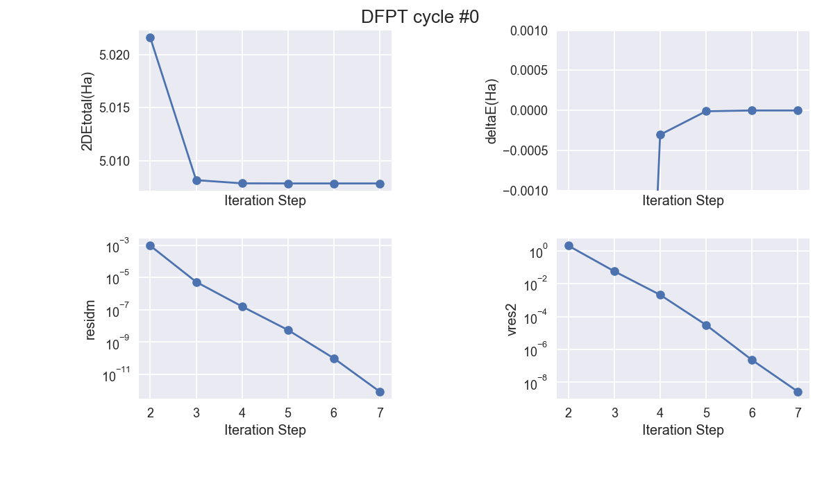
4 DFPT calculation of the dynamical matrix at $\Gamma$

We are now in the position to compute the full dynamical matrix at the $\Gamma$ point (q=0). You can copy the file $ABI_TESTS/tutorespfn/Input/trf1_4.abi in Work_rf1. This is your input file.

As for test rf1_3, the changes with respect to trf1_1.abi are all gathered in the first part of this file. Moreover, the changes with respect to trf1_3.abi concern only the input variables rfatpol, and rfdir. Namely, all the atoms will be displaced, in all the directions.

Warning

You need to copy trf1_1o_WFK to trf1_4i_WFK so Abinit can find the wavefunction during the calculation.

View tests/tutorespfn/Input/trf1_4.abi

There are six perturbations to consider. So, one might think that the CPU time will raise accordingly. This is not true, as ABINIT is able to determine which perturbations are the symmetric of another perturbation, see section 3 of the respfn help file.

Now, you can make the run. You open the file trf1_4.abo, and notice that the response to two perturbations were computed explicitly, while the response to the other four could be deduced from the two first by using the symmetries.

 The list of irreducible perturbations for this q vector is:
    1)    idir= 1    ipert=   1
    2)    idir= 1    ipert=   2

Nothing mysterious: one of the two irreducible perturbations is for the Al atom, placed in a rather symmetric local site, and the other perturbation is for the As atom.

The phonon frequencies, obtained by diagonalizing the dynamical matrix (where the atomic masses have been taken into account, see amu), are given as follows:

   Phonon wavevector (reduced coordinates) :  0.00000  0.00000  0.00000
  Phonon energies in Hartree :
    0.000000E+00  0.000000E+00  0.000000E+00  1.568561E-03  1.568561E-03
    1.568561E-03
  Phonon frequencies in cm-1    :
 -  0.000000E+00  0.000000E+00  0.000000E+00  3.442594E+02  3.442594E+02
 -  3.442594E+02

Tip

You might wonder about the dash sign present in the first column of the two lines giving the frequencies in cm$^{-1}$. The first column of the main ABINIT output files is always dedicated to signs needed to automatically treat the comparison with respect to reference files. Except if you become an ABINIT developer, you should ignore these signs. In the present case, they should not be interpreted as a minus sign for the floating numbers that follow them…

There is a good news and a bad news about this result. The good news is that there are indeed three acoustic modes, with frequency exactly zero. This has been obtained thanks to the imposition of the acoustic sum rule, with the default value of the variable asr.

By the way, switching asr to zero delivers

  Phonon wavevector (reduced coordinates) :  0.00000  0.00000  0.00000
 Phonon energies in Hartree :
   2.559712E-06  2.559712E-06  2.559713E-06  1.568567E-03  1.568567E-03
   1.568567E-03
 Phonon frequencies in cm-1    :
-  5.617917E-01  5.617918E-01  5.617921E-01  3.442606E+02  3.442606E+02
-  3.442606E+02

The three acoustic modes do not have exactly zero frequency, still these are less less than 1 cm$^{-1}$, which is rather good! The other modes are marginally modified by the imposition of the acoustic sum rule.

The bad news comes when the three other frequencies are compared with experimental results, or other theoretical results. Indeed, in the present run, one obtains three degenerate modes, while there should be a (2+1) splitting. This can be seen in the paper Ab initio calculation of phonon dispersions in semiconductors [Giannozzi1991], especially Fig. 2.

Actually, we have forgotten to take into account the coupling between atomic displacements and the homogeneous electric field, that exists in the case of polar insulators, for so-called “Longitudinal Optic (LO) modes”. A splitting appears between these modes and the “Transverse Optic (TO) modes”. This splitting (Lyddane-Sachs-Teller LO-TO splitting) is presented in simple terms in standard textbooks, and should not be forgotten in doing Ab initio calculations of phonon frequencies.

Thus we have now to treat correctly the homogeneous electric field type perturbation.

5 DFPT calculation of the effect of an homogeneous electric field

The treatment of the homogeneous electric field perturbation is formally much more complex than the treatment of atomic displacements. This is primarily because the change of potential associated with an homogeneous electric field is not periodic, and thus does not satisfy the Born-von Karman periodic boundary conditions.

For the purpose of the present tutorial, one should read the section II.C of the above-mentioned paper [Giannozzi1991]. The reader will find in [Gonze1997] and [Gonze1997a] more detailed information about this perturbation, closely related to the ABINIT implementation. There is also an extensive discussion of the Born effective charges by [Ghosez1998].

In order to compute the response of solids to an homogeneous electric field in ABINIT, the remaining sections of the respfn help file should be read. These sections also present the information needed to compute phonons with non-zero q wavevector, which will be the subject of the next section of the present tutorial. The sections to be read are:

• the part of section 1 that had not yet been read
• section 2
• section 4
• and, for completeness, section 5

You are now in the position to compute the full dynamical matrix at $\Gamma$ (q=0), including the coupling with an homogeneous electric field. You can copy $ABI_TESTS/tutorespfn/Input/trf1_5.abi in Work_rf1. This is your input file.

View tests/tutorespfn/Input/trf1_5.abi View tests/tutorespfn/Refs/trf1_5.abo

As for the other DFPT tests, the changes with respect to the trf1_1.abi are all gathered in the first part of this file. Unlike the other tests, however, the multi-dataset mode was used, computing from scratch the ground-state properties, then computing the effect of the ddk perturbation, then the effect of all other perturbations (electric field as well as atomic displacements).

The analysis of the output file is even more cumbersome than the previous ones. Let us skip the first dataset. In the dataset 2 section, one perturbation is correctly selected:

 ==>  initialize data related to q vector <==

 The list of irreducible perturbations for this q vector is:
    1)    idir= 1    ipert=   3

================================================================================

--------------------------------------------------------------------------------
 Perturbation wavevector (in red.coord.)   0.000000  0.000000  0.000000
 Perturbation : derivative vs k along direction   1

The analysis of the output for this particular perturbation is not particularly interesting, except for the f-sum rule ratio

 dfpt_looppert : ek2=    1.6833336546E+01
          f-sum rule ratio=    1.0028274804E+00

that should be close to 1, and becomes closer to it when ecut is increased, and the sampling of k points is improved. (In the present status of ABINIT, the f-rule ratio is not computed correctly when ecutsm/=0)

In the third dataset section, three irreducible perturbations are considered:

 ==>  initialize data related to q vector <==

 The list of irreducible perturbations for this q vector is:
    1)    idir= 1    ipert=   1
    2)    idir= 1    ipert=   2
    3)    idir= 1    ipert=   4

Much later, the dielectric tensor is given:

  Dielectric tensor, in cartesian coordinates,
     j1       j2             matrix element
  dir pert dir pert     real part    imaginary part

   1    4   1    4         9.7501435881        -0.0000000000
   1    4   2    4         0.0000000000        -0.0000000000
   1    4   3    4         0.0000000000        -0.0000000000

   2    4   1    4         0.0000000000        -0.0000000000
   2    4   2    4         9.7501435881        -0.0000000000
   2    4   3    4         0.0000000000        -0.0000000000

   3    4   1    4         0.0000000000        -0.0000000000
   3    4   2    4         0.0000000000        -0.0000000000
   3    4   3    4         9.7501435881        -0.0000000000

It is diagonal and isotropic, and corresponds to a dielectric constant of 9.7501435881.

Then, the Born effective charges are given, either computed from the derivative of the wavefunctions with respect to the electric field, or computed from the derivative of the wavefunctions with respect to an atomic displacement, as explained in section II of [Gonze1997a]:

  Effective charges, in cartesian coordinates,
  (from electric field response)
  ...

and

  Effective charges, in cartesian coordinates,
  (from phonon response)
  ...

Namely, the Born effective charge of the Al atom is 2.105, and the one of the As atom is -2.127. The charge neutrality sum rule is not fulfilled exactly. When ecut is increased, and the sampling of k points is improved, the sum of the two charges goes closer to zero.

Finally, the phonon frequencies are computed:

  Phonon wavevector (reduced coordinates) :  0.00000  0.00000  0.00000
 Phonon energies in Hartree :
   2.559710E-06  2.559710E-06  2.559711E-06  1.568567E-03  1.568567E-03
   1.568567E-03
 Phonon frequencies in cm-1    :
-  5.617914E-01  5.617914E-01  5.617917E-01  3.442606E+02  3.442606E+02
-  3.442606E+02

  Phonon at Gamma, with non-analyticity in the
  direction (cartesian coordinates)  1.00000  0.00000  0.00000
 Phonon energies in Hartree :
   2.559710E-06  2.559710E-06  4.044009E-06  1.568567E-03  1.568567E-03
   1.729799E-03
 Phonon frequencies in cm-1    :
-  5.617914E-01  5.617914E-01  8.875575E-01  3.442606E+02  3.442606E+02
-  3.796470E+02

  Phonon at Gamma, with non-analyticity in the
  direction (cartesian coordinates)  0.00000  1.00000  0.00000
 Phonon energies in Hartree :
   2.559710E-06  2.559711E-06  4.044009E-06  1.568567E-03  1.568567E-03
   1.729799E-03
 Phonon frequencies in cm-1    :
-  5.617914E-01  5.617917E-01  8.875573E-01  3.442606E+02  3.442606E+02
-  3.796470E+02

  Phonon at Gamma, with non-analyticity in the
  direction (cartesian coordinates)  0.00000  0.00000  1.00000
 Phonon energies in Hartree :
   2.559710E-06  2.559711E-06  4.044008E-06  1.568567E-03  1.568567E-03
   1.729799E-03
 Phonon frequencies in cm-1    :
-  5.617914E-01  5.617917E-01  8.875573E-01  3.442606E+02  3.442606E+02
-  3.796470E+02

There are four sections. In the first one, any effect of the homogeneous electric field is simply discarded, while the three next sections the electric field is considered along the three cartesian coordinates.

In the present material, the directionality of the electric field has no influence. We note that there are still three acoustic mode, below 1 cm$^{-1}$, while the optic modes have the correct degeneracies: two TO modes at 344.3 cm$^{-1}$, and one LO mode at 379.6 cm$^{-1}$.

These values can be compared to experimental (361 cm$^{-1}$, 402 cm$^{-1}$) as well as theoretical (363 cm$^{-1}$, 400 cm$^{-1}$) values (again [Giannozzi1991]). Most of the discrepancy comes from the too low value of ecut. Using ABINIT with ecut=6 Hartree gives (358.8 cm$^{-1}$, 389.8 cm$^{-1}$). The remaining of the discrepancy may come partly from the pseudopotentials, that are particularly soft.

The comparison of Born effective charges is also interesting. After imposition of the neutrality sum rule, the Al Born effective charge is 2.116. The value from Gianozzi et al is 2.17, the experimental value is 2.18. Increasing ecut to 6 Hartree in ABINIT gives 2.168.

For the dielectric tensor, it is more delicate. The value from Gianozzi et al is 9.2, while the experimental value is 8.2 . The agreement is not very good, a fact that can be attributed to the DFT lack of polarization-dependence [Gonze1995a]. Still, the agreement of our calculation with the theoretical result is not very good. With ecut = 3 Hartree, we have 9.75. Changing it to 6 Hartree gives 10.40 . A better k point sampling (8x8x8), with ecut = 6 Hartree, reduces the value to 9.89. Changing pseudopotentials finally improves the agreement: with the much harder al.psp8 and as.psp8 pseudopotentials with adequate ecut = 20 Hartree and 8x8x8 Monkhorst-Pack sampling, we reach a value of 9.30. Note that we need to change ixc=-1012 and consider nband=9, since there is 3 electrons for Al and 15 electrons for As moving in these pseudopotential. This information can be found by searching zion in the .abo of any file using the pseudopotentials. This illustrates that the dielectric tensor is a much more sensitive quantity than the others.

6 DFPT calculation of phonon frequencies at non-zero q

The computation of phonon frequencies at non-zero q is actually simpler than the one at $\Gamma$. One must distinguish two cases. Either the q wavevector connects k points that belong to the same grid, or the wavevector q is general. In any case, the computation within the reciprocal space DFPT formalism is more efficient than the real space frozen-phonon technique since the use of supercells is completely avoided with DFPT. For an explanation of this fact, see for example section IV of [Gonze1997].

You can copy the file $ABI_TESTS/tutorespfn/Input/trf1_6.abi in Work_rf1. This is your input file.

View tests/tutorespfn/Input/trf1_6.abi View tests/tutorespfn/Refs/trf1_6.abo

As for the other RF tests, the changes with respect to trf1_1.abi are all gathered in the first part of this file. The multi-dataset mode is used, computing from scratch the ground-state wave functions, then computing different dynamical matrices with DFPT. The run is about 1 minutes on a 2.8 GHz machine. In the mean time, you might read more of the ABINIT documentation (why not the mrgddb_help and the anaddb_help).

The results of this simulation can be compared to those provided in [Giannozzi1991]. The agreement is rather good, despite the low cut-off energy, and different pseudopotentials.

At X, they get 95 cm$^{-1}$, 216 cm$^{-1}$, 337 cm$^{-1}$ and 393 cm$^{-1}$, while we get 92.8 cm$^{-1}$, 204.6 cm$^{-1}$, 313.8 cm$^{-1}$ and 375.9 cm$^{-1}$. With ecut=6 Hartree, we get 89.7 cm$^{-1}$, 212.3 cm$^{-1}$, 328.5 cm$^{-1}$ and 385.8 cm$^{-1}$.

At L, they get 71 cm$^{-1}$, 212 cm$^{-1}$, 352 cm$^{-1}$ and 372 cm$^{-1}$, while we get 69.2 cm$^{-1}$, 202.5 cm$^{-1}$, 332.6 cm$^{-1}$ and 352.3 cm$^{-1}$. With ecut=6 Hartree, we get 68.1 cm$^{-1}$, 208.5 cm$^{-1}$, 346.7 cm$^{-1}$ and 362.6 cm$^{-1}$.

At q=(0.1 0 0), we get 31.7 cm$^{-1}$, 63.6 cm$^{-1}$, 342.0 cm$^{-1}$ and 379.7 cm$^{-1}$. The acoustic modes tends (nearly-)linearly to zero, while the optic modes are close to their values at $\Gamma$ : 344.3 cm$^{-1}$ and 379.6 cm$^{-1}$.

---

Note

This ABINIT tutorial is now finished. You are advised to go through the second tutorial on DFPT to make some post-processing analysis (phonon dispersions, thermodynamical properties, etc)