Second tutorial on the Projector Augmented-Wave (PAW) technique¶

Generation of PAW atomic datasets¶

This tutorial aims at showing how to create your own atomic datasets for the Projector Augmented-Wave (PAW) method.

You will learn how to generate these atomic datasets and how to control their softness and transferability. You already should know how to use ABINIT in the PAW case (see the tutorial PAW1 ).

This tutorial should take about 2h00.

Note

Supposing you made your own installation of ABINIT, the input files to run the examples are in the ~abinit/tests/ directory where ~abinit is the absolute path of the abinit top-level directory. If you have NOT made your own install, ask your system administrator where to find the package, especially the executable and test files.

In case you work on your own PC or workstation, to make things easier, we suggest you define some handy environment variables by executing the following lines in the terminal:

export ABI_HOME=Replace_with_absolute_path_to_abinit_top_level_dir # Change this line
export PATH=$ABI_HOME/src/98_main/:$PATH      # Do not change this line: path to executable
export ABI_TESTS=$ABI_HOME/tests/             # Do not change this line: path to tests dir
export ABI_PSPDIR=$ABI_TESTS/Pspdir/  # Do not change this line: path to pseudos dir

Examples in this tutorial use these shell variables: copy and paste the code snippets into the terminal (remember to set ABI_HOME first!) or, alternatively, source the set_abienv.sh script located in the ~abinit directory:

source ~abinit/set_abienv.sh

The ‘export PATH’ line adds the directory containing the executables to your PATH so that you can invoke the code by simply typing abinit in the terminal instead of providing the absolute path.

To execute the tutorials, create a working directory (Work*) and copy there the input files of the lesson.

Most of the tutorials do not rely on parallelism (except specific tutorials on parallelism). However you can run most of the tutorial examples in parallel with MPI, see the topic on parallelism.

1. The PAW atomic dataset - introduction¶

The PAW method is based on the definition of spherical augmentation regions of radius $r_c$ around the atoms of the system in which a basis of atomic partial-waves $\phi_i$, of pseudized partial-waves $\tphi_i$, and of projectors $\tprj_i$ (dual to $\tphi_i$) have to be defined. This set of partial-waves and projectors functions (and some additional atomic data) are stored in a so-called PAW dataset. A PAW dataset has to be generated for each atomic species in order to reproduce atomic behavior as accurate as possible while requiring minimal CPU and memory resources in executing ABINIT for the crystal simulations. These two constraints are obviously conflicting.

The PAW dataset generation is the purpose of this tutorial. It is done according the following procedure (all parameters that define a PAW dataset are in bold):

Choose and define the concerned chemical species (name and atomic number).
Solve the atomic all-electrons problem in a given atomic configuration. The atomic problem is solved within the DFT formalism, using an exchange-correlation functional and either a Schrodinger (default) or scalar-relativistic approximation. This spherical problem is solved on a radial grid. The atomic problem is solved for a given electronic configuration that can be an ionized/excited one.
Choose a set of electrons that will be considered as frozen around the nucleus (core electrons). The others electrons are valence ones and will be used in the PAW basis. The core density is then deduced from the core electrons wave functions. A smooth core density equal to the core density outside a given $r_{core}$ matching radius is computed.
Choose the size of the PAW basis (number of partial-waves and projectors). Then choose the partial-waves included in the basis. The later can be atomic eigen-functions related to valence electrons (bound states) and/or additional atomic functions, solution of the wave equation for a given $l$ quantum number at arbitrary reference energies (unbound states).
Generate pseudo partial-waves (smooth partial-waves build with a pseudization scheme and equal to partial-waves outside a given $r_c$ matching radius) and associated projector functions. Pseudo partial-waves are solutions of the PAW Hamiltonian deduced from the atomic Hamiltonian by pseudizing the effective potential (a local pseudopotential is built and equal to effective potential outside a $r_{Vloc} matching radius). Projectors and partial-waves are then orthogonalized with a chosen orthogonalization scheme.
Build a compensation charge density used later in order to retrieve the total charge of the atom. This compensation charge density is located inside the PAW spheres and based on an analytical shape function (which analytic form and localization radius $r_{shape}$ can be chosen).

The user can choose between two PAW dataset generators to produce atomic files directly readable by ABINIT. The first one is the PAW generator ATOMPAW (originally by N. Holzwarth) and the second one is the Ultra-Soft USPP generator (originally written by D. Vanderbilt). In this tutorial, we concentrate only on ATOMPAW.

It is highly recommended to refer to the following papers to understand correctly the generation of PAW atomic datasets:

“Projector augmented-wave method” - [Bloechl1994]
“A projector Augmented Wave (PAW) code for electronic structure” - [Holzwarth2001]
“From ultrasoft pseudopotentials to the projector augmented-wave method” - [Kresse1999]
“Electronic structure packages: two implementations of the Projector Augmented-Wave (PAW) formalism” - [Torrent2010]
“Notes for revised form of atompaw code” (by N. Holzwarth) - PDF

2. Use of the generation code¶

Before continuing, you might consider to work in a different subdirectory as for the other tutorials. Why not Work_paw2?

cd $ABI_TESTS/tutorial/Input
mkdir Work_paw2
cd Work_paw2

You have now to install the ATOMPAW code. In your internet browser, enter the following URL:

 https://users.wfu.edu/natalie/papers/pwpaw/

Then, download the last version of the tar.gz file, unzip and untar it. Enter the atompaw-4.x.y.z and execute:

    mkdir build
    cd build
    ../configure
    make

if all goes well, you get the ATOMPAW executable at atompaw-4.x.y.z/build/src/atompaw.
If not, Go into the directory doc, open the file atompaw-usersguide.pdf, go p.3 and follow the instructions.

Note

On MacOS, you can use homebrew package manager and install ATOMPAW by typing:

        brew install atompaw/repo/atompaw

Note

In the following, we name atompaw the ATOMPAW executable.

How to use ATOMPAW?

The following process will be applied to Nickel in the next paragraph:

Edit an input file in a text editor (content of input explained here)
Run: atompaw < inputfile

Partial waves $\phi_i$, PS partial-waves $\tphi_i$ and projectors $\tprj_i$ are given in wfn.i files. Logarithmic derivatives from atomic Hamiltonian and PAW Hamiltonian resolutions are given in logderiv.l files. A summary of the atomic all-electron computation and PAW dataset properties can be found in the Atom_name file (Atom_name is the first parameter of the input file).

Resulting PAW dataset is contained in:

Atom_name.XCfunc.xml file
Normalized XML file according to the PAW- XML specifications (recommended).
Atom_name.XCfunc-paw.abinit file
Proprietary legacy format for ABINIT

3. First (and basic) PAW dataset for Nickel¶

Our test case will be nickel; electronic configuration: $[1s^2 2s^2 2p^6 3s^2 3p^6 3d^8 4s^2 4p^0]$.

In a first stage, copy a simple input file for ATOMPAW in your working directory (find it in $ABI_HOME/doc/tutorial/paw2/paw2_assets/Ni.atompaw.input1). Edit this file.

This file has been built in the following way:

All-electron calculation parameters:
- 1^st line: define the material.
```
    Ni 28
```
- 2^nd line: choose the exchange-correlation functional (LDA-PW or GGA-PBE) and select a scalar-relativistic wave equation (nonrelativistic or scalarrelativistic) and a (2000 points) logarithmic grid.
```
    GGA-PBE scalarrelativistic loggrid 2000
```
Electronic configuration: How many electronic states do we need to include in the computation? Besides the fully and partially occupied states, it is recommended to add all states that could be reached by electrons in the solid. Here, for Nickel, the $4p$ state is concerned. So we decide to add it in the computation.
- 3^rd line: define the electronic configuration. A line with the maximum $n$ quantum number for each electronic shell; here 4 4 3 means 4s, 4p, 3d.
```
    4 4 3 0 0 0
```
- Following lines : definition of occupation numbers. For each partially occupied shell enter the occupation number. An excited configuration may be useful if the PAW dataset is intended for use in a context where the material is charged (such as oxides). Although, in our experience, the results are not highly dependent on the chosen electronic configuration. We choose here the $[3d^8 4s^2 4p^0]$ configuration. Only $3d$ and $4p$ shells are partially occupied (3 2 8 and 4 1 0 lines). A 0 0 0 ends the occupation section.
```
    3 2 8
    4 1 0
    0 0 0
```
Selection of core and valence electrons. In a first approach, select only electrons from outer shells as valence. But, if particular thermodynamical conditions are to be simulated, it is generally needed to include “semi-core states” in the set of valence electrons. Semi-core states are generally needed with transition metal and rare-earth materials. Note that all wave functions designated as valence electrons will be used in the partial-wave basis. Core shells are designated by a $c$ and valence shells by a $v$. All $s$ states first, then $p$ states and finally $d$ states. Here:
```
    c
    c
    c
    v
    c
    c
    v
    v
```
means:
```
    1s core
    2s core
    3s core
    4s valence
    2p core
    3p core
    4p valence
    3d valence
```
Partial-waves basis generation:
- A line with $l_{max}$ the maximum $l$ for the partial-waves basis. Here $l_{max}=2$.
```
    2
```
- A line with the $r_{PAW}$ radius.
  Select it to be slightly less than half the inter-atomic distance in the solid (as a first choice). Here $r_{PAW}=2.3\ a.u$.
```
    2.3
```
- Next lines: add additional partial-waves $\phi_i$ if needed. Choose to have 2 partial-waves per angular momentum in the basis (this choice is not necessarily optimal but this is the most common one; if $r_{PAW}$ is small enough, 1 partial-wave per $l$ may suffice). As a first guess, put all reference energies for additional partial-waves to 0 Rydberg. For each angular momentum, first add “y” to add an additional partial-wave. Then, next line, put the value in Rydberg units. Repeat this for each new partial-wave and finally put “n”. Note : For each angular momentum, valence states already are included in the partial-waves basis. Here $4s$, $4p$ and $3d$ states already are in the basis. In the present file:
```
    y
    0.5
    n
```
  means that an additional $s$- partial-wave at $E_{ref}=0.5$ Ry as been added,
```
    y
    1.
    n
```
  means that an additional $p$- partial-wave at $E_{ref}=1.$ Ry has been added,
```
    y
    1.
    n
```
  means that an additional $d$- partial-wave at $E_{ref}=1.$ Ry as been added. Finally, partial-waves basis contains two $s$-, two $p$- and two $d$- partial-waves.
- Next line: definition of the generation scheme for pseudo partial waves $\tphi_i$, and of projectors $\tprj_i$. We begin here with a simple scheme (i.e. “Bloechl” scheme, proposed by P. Blochl [Bloechl1994]). This will probably be changed later to make the PAW dataset more efficient.
```
    bloechl
```
- Next line: generation scheme for local pseudopotential $V_{loc}$. In order to get PS partial-waves, the atomic potential has to be “pseudized” using an arbitrary pseudization scheme. We choose here a “Troullier-Martins” using a wave equation at $l_{loc}=3$ and $E_{loc}=0.$ Ry. As a first draft, it is always recommended to put $l_{loc}=1+l_{max}$.
```
    3 0. troulliermartins
```
- Next two lines: XMLOUT makes ATOMPAW generate a PAW dataset in XML format; The next line contains options for this ABINIT file. “default” set all parameters to their default value.
```
    XMLOUT
    default
```
- The END keyword ends the file.
```
    END
```

At this stage, run ATOMPAW. For this purpose, simply enter:

atompaw < Ni.atompaw.input1

Lot of files are produced. We will examine some of them. A summary of the PAW dataset generation process has been written in a file named Ni.
Open it. It should look like:

 Completed calculations for Ni
 Exchange-correlation type: GGA, Perdew-Burke-Ernzerhof
  Radial integration grid is logarithmic 
r0 =   2.2810899E-04 h =   6.3870518E-03   n =      2000 rmax =   8.0000000E+01
 Scalar relativistic calculation
   AEatom converged in          32  iterations
     for nz =  28.00
     delta  =    9.5504321957145377E-017
  All Electron Orbital energies:         
  n  l     occupancy       energy
 1  0      2.0000000E+00 -6.0358607E+02
 2  0      2.0000000E+00 -7.2163318E+01
 3  0      2.0000000E+00 -8.1627107E+00
 4  0      2.0000000E+00 -4.1475541E-01
 2  1      6.0000000E+00 -6.2083048E+01
 3  1      6.0000000E+00 -5.2469208E+00
 4  1      0.0000000E+00 -9.0035739E-02
 3  2      8.0000000E+00 -6.5223644E-01

  Total energy
     Total                    :    -3041.0743834110435     
 Completed calculations for Ni
 Exchange-correlation type: GGA, Perdew-Burke-Ernzerhof
  Radial integration grid is logarithmic 
r0 =   2.2810899E-04 h =   6.3870518E-03   n =      2000 rmax =   8.0000000E+01
 Scalar relativistic calculation
   SCatom converged in           1  iterations
     for nz =  28.00
     delta  =    8.7786021384577619E-017
   Valence Electron Orbital energies:         
  n  l     occupancy       energy
 4  0      2.0000000E+00 -4.1475541E-01
 4  1      0.0000000E+00 -9.0035739E-02
 3  2      8.0000000E+00 -6.5223644E-01

  Total energy
     Total                    :    -3041.0743834029249     
     Valence                  :    -185.18230020196870     
  paw parameters: 
       lmax =            2
         rc =    2.3096984974114871     
        irc =         1445
 Vloc: Norm-conserving Troullier-Martins with l= 3;e=   0.0000E+00
 Projector type: Bloechl + Gram-Schmidt ortho.
 Sinc^2 compensation charge shape zeroed at rc

Number of basis functions     6
 No.   n    l      Energy         Cp coeff         Occ
    1    4    0 -4.1475541E-01 -9.5091487E+00  2.0000000E+00
    2  999    0  5.0000000E-01  3.2926948E+00  0.0000000E+00
    3    4    1 -9.0035739E-02 -8.9594191E+00  0.0000000E+00
    4  999    1  1.0000000E+00  1.0610645E+01  0.0000000E+00
    5    3    2 -6.5223644E-01  9.1576184E+00  8.0000000E+00
    6  999    2  0.0000000E+00  1.3369076E+01  0.0000000E+00
 Completed diagonalization of ovlp with info =        0

 Eigenvalues of overlap operator (in the basis of projectors):
    1        7.27257365E-03
    2        2.25491432E-02
    3        1.25237568E+00
    4        1.87485118E+00
    5        1.05720648E+01
    6        2.00807906E+01

  Summary of PAW energies
        Total valence energy       -185.18230536120760     
          Smooth energy             11.667559552612433     
          One center               -196.84986491382003     
          Smooth kinetic            15.154868503980399     
          Vloc energy              -2.8094614733964467     
          Smooth exch-corr         -3.3767012052640886     
          One-center xc            -123.07769380742522

The generated PAW dataset (contained in Ni.GGA-PBE.xml file) is a first draft. Several parameters have to be adjusted, in order to get accurate results and efficient DFT calculations.

Note

The Ni.GGA-PBE.xml file is directly usable by ABINIT.

4. Checking the sensitivity to some parameters¶

4.a. The radial grid¶

Let’s try to select 700 points in the logarithmic grid and check if any noticeable difference in the results appears. You just have to replace 2000 by 700 in the second line of Ni.atompaw.input1 file.
Then run:

atompaw < Ni.atompaw.input1

again and look at the Ni file:

   Summary of PAW energies
         Total valence energy       -185.18230027710337     
           Smooth energy             11.634042318422193     
           One center               -196.81634259552555     
           Smooth kinetic            15.117782033814152     
           Vloc energy              -2.8024659321861067     
           Smooth exch-corr         -3.3712015132649102     
           One-center xc            -123.08319475096027

As you see, results obtained with this new grid are very close to previous ones, expecially the valence energy. We can keep the 700 points grid.

Note

We could try to decrease the size of the grid. Small grids give PAW dataset with small size (in kB) and run faster in ABINIT, but accuracy can be affected.

Note

The final $r_{PAW}$ value (rc = ... in Ni file) changes with the grid; just because $r_{PAW}$ is adjusted in order to belong exactly to the radial grid. By looking in ATOMPAW user’s guide, you can choose to keep it constant.

4.b. The relativistic approximation of the wave equation¶

The scalar-relativistic option should give better results than non-relativistic one, but it sometimes produces difficulties for the convergence of the atomic problem (either at the all-electron resolution step or at the PAW Hamiltonian solution step). If convergence cannot be reached, try a non-relativistic calculation (not recommended for high Z materials).

Note

For the following, note that you always should check the Ni file, especially the values of valence energy. You can find the valence energy computed for the exact atomic problem and the valence energy computed with the PAW parameters. These two results should be in close agreement!

5. Adjusting partial-waves and projectors¶

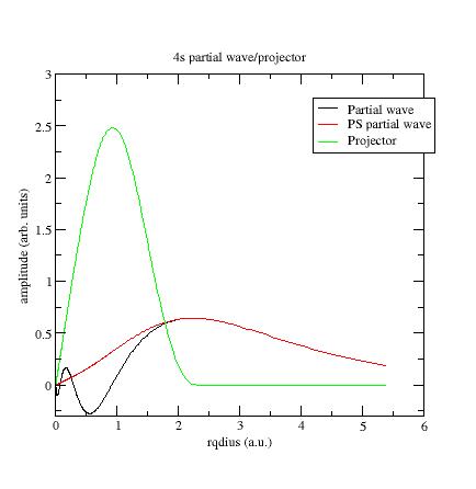
Examine the AE partial-waves $\phi_i$, PS partial-waves $\tphi_i$ and projectors $\tprj_i$. These are saved in files named wfni, where i ranges over the number of partial-waves used, so 6 in the present example. Each file contains 4 columns: the radius $r$ in column 1, the AE partial-wave $\phi_i(r)$ in column 2, the PS partial-wave $\tphi_i(r)$ in column 3, and the projector $\tprj_i(r)$ in column 4.
Plot the 3 curves as a function of radius using a plotting tool of your choice.

Below the first $s$- partial-wave /projector of the Ni example:

First s partial-wave

$\phi_i$ should meet $\tphi_i$ near or after the last maximum (or minimum). If not, it is preferable to change the value of the matching (pseudization) radius $r_c$.
The maxima of $\tphi_i$ and $\tprj_i$ functions should roughly have the same order of magnitude. If not, you can try to get this in three ways:
1. Change the matching radius for this partial-wave; but this is not always possible (PAW spheres should not overlap in the solid).
2. Change the pseudopotential scheme (see later).
3. If there are two (or more) partial-waves for the angular momentum $l$ under consideration, decreasing the magnitude of the projector is possible by displacing the references energies. Moving the energies away from each other generally reduces the magnitude of the projectors, but too big a difference between energies can lead to wrong logarithmic derivatives (see following section).

Example: plot the wfn6 file, related to the second $d$- partial-wave:

2nd d partial-wave

This partial-wave has been generated at $E_{ref}=0$ Ry and orthogonalized with the first $d$- partial-wave which has an eigenenergy equal to $-0.65$ Ry (see Ni file). These two energies are too close and orthogonalization process produces “high” partial-waves. Try to replace the reference energy for the additional $d$- partial-wave. For example, put $E_{ref}=1.$ Ry instead of $E_{ref}=0.$ Ry (line 24 of Ni.atompaw.input1 file).

Run ATOMPAW again and plot wfn6 file:

2nd d partial-wave

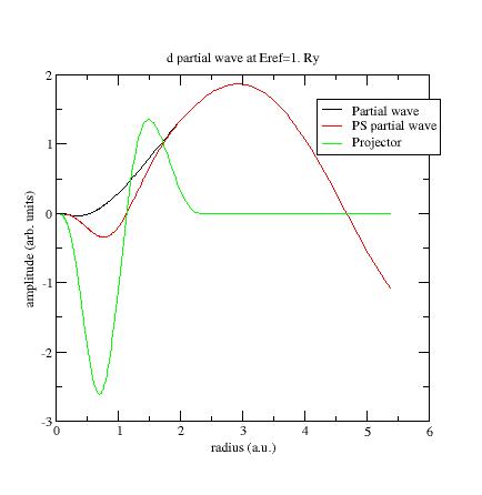
Now the PS partial-wave and projector have the same order of magnitude!

Important

Note again that you should always check the two Valence energy values in Ni file and make sure they are as close as possible. If not, choices for projectors and/or partial-waves are certainly not judicious.

6. Examine the logarithmic derivatives¶

Examine the logarithmic derivatives, i.e., derivatives of an $l$-state $\frac{d(log(\Psi_l(E))}{dE}$ computed for the exact atomic problem and with the PAW dataset. They are printed in the logderiv.l files. Each logderiv.l file corresponds to an angular momentum $l$ and contains five columns of data: the energy, the logarithmic derivative of the $l$-state of the exact atomic problem, the logarithmic derivative of the pseudized problem (and two other colums not relevant for this section). In the following, when you edit a logderiv file, only edit the three first columns.
In our Ni example, $l=0$, $1$ or $2$.

The logarithmic derivatives should have the following properties:

The 2 curves should be superimposed as much as possible. By construction, they are superimposed at the 2 energies corresponding to the 2 $l$ partial-waves. If the superimposition is not good enough, the reference energy for the second $l$ partial-wave should be changed.
Generally a discontinuity in the logarithmic derivative curve appears at $0$ Ry $\le E_0\le 4$ Ry. A reasonable choice is to choose the 2 reference energies so that $E_0$ is in between.
Too close reference energies produce “hard” projector functions (see section 5). But moving reference energies away from each other can damage accuracy of logarithmic derivatives

Here are the three logarithmic derivative curves for the current dataset:

l=0 log derivatives

l=1 logderivatives

l=2 logderivatives

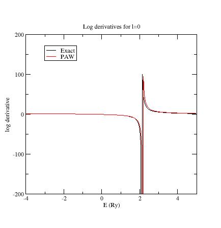
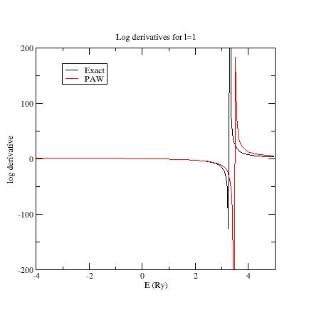
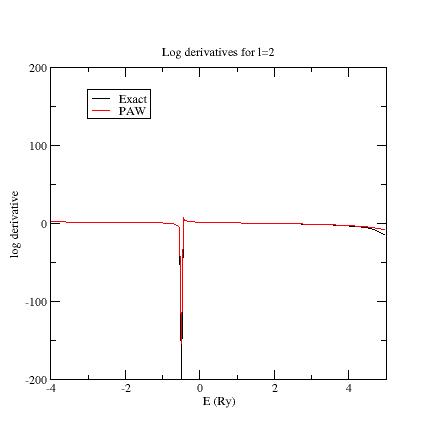
As you can see, except for $l=2$, exact and PAW logarithmic derivatives do not match!
According to the previous remarks, try other values for the references energies of the $s$- and $p$- additional partial-waves.
First, edit again the Ni.atompaw.input1 file and put $E_{ref}=3$ Ry for the additional $s$- state (line 18); run ATOMPAW again. Plot the logderiv.0 file. You should get:

l=0 log derivatives

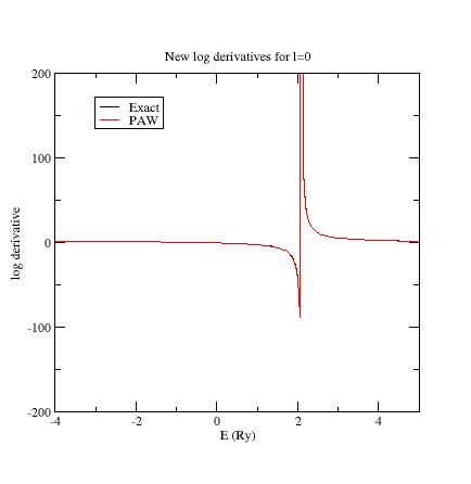
Then put $E_{ref}=4$ Ry for the second $p$- state (line 21); run ATOMPAW again. Plot again the logderiv.1 file.
You should get:

l=1 log derivatives

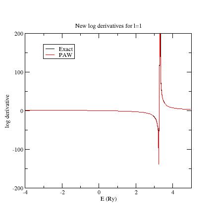
Now, all PAW logarithmic derivatives match with the exact ones in a reasonable interval.

Note

It is possible to change the interval of energies used to plot logarithmic derivatives (default is $[-5;5]$) and also to compute them at more points (default is $200$). Just add the following keywords at the end of the SECOND LINE of the input file if you want ATOMPAW to output logarithmic derivatives for energies in [-10;10] at 500 points:

    logderivrange -10 10 500

Additional information related to logarithmic derivatives: ghost states

Another possible issue could be the presence of a discontinuity in the PAW logarithmic derivative curve at an energy where the exact logarithmic derivative is continuous. This generally shows the presence of a ghost state.

First, try to change to value of reference energies; this sometimes can make the ghost state disappear.
If not, it can be useful to change the pseudopotential scheme. Norm-conserving pseudopotentials are sometimes too attractive near $r=0$.
- A 1^st solution is to change the quantum number used to generate the norm-conserving pseudopotential. But this is generally not sufficient.
- A 2^nd solution is to select a ultrasoft pseudopotential, freeing the norm conservation constraint (simply replace troulliermartins by ultrasoft in the input file).
- A 3^rd solution is to select a simple bessel pseudopotential (replace troulliermartins by bessel in the input file). But, in that case, one has to noticeably decrease the matching radius $r_{Vloc}$ if one wants to keep reasonable physical results. Selecting a value of $r_{Vloc}$ between $0.6~r_{PAW}$ and $0.8~r_{PAW}$ is a good choice. To change the value of $r_{Vloc}$, one has to explicitely put all matching radii: $r_{PAW}$, $r_{shape}$, $r_{Vloc}$ and $r_{core}$; see user’s guide.
Last solution : try to change the matching radius $r_c$ for one (or both) $l$ partial-wave(s). In some cases, changing $r_c$ can remove ghost states.

In most cases (changing pseudopotential or matching radius), one has to restart the procedure from step 5.

To see an example of ghost state, use the $ABI_HOME/doc/tutorial/paw2_assets/Ni.ghost.atompaw.input file and run it with ATOMPAW.

Look at the $l=1$ logarithmic derivatives (logderiv.1 file). They look like:

Ni l=1 log derivatives

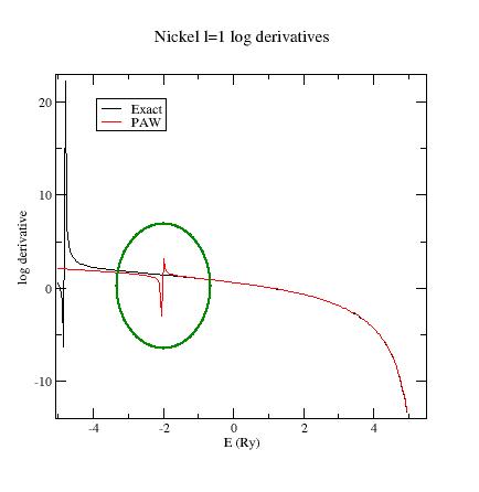
Now, edit the Ni.ghost.atompaw.input file and replace troulliermartins by ultrasoft.
Run ATOMPAW again… and look at logderiv.1 file. The ghost state has moved!

Edit again the file and replace troulliermartins by bessel (line 28); then change the 17^th line 2.0 2.0 2.0 2.0 by 2.0 2.0 1.8 2.0 (decreasing the $r_{Vloc}$ radius from $2.0$ to $1.8$).
Run ATOMPAW: the ghost state disappears!

Start from the original state of Ni.ghost.atompaw.input file and put 1.6 for the matching radius of $p$- states (put 1.6 on lines 31 and 32). Run ATOMPAW: the ghost state disappears!

7. Testing the “efficiency” of a PAW dataset¶

Let’s use again our Ni.atompaw.input1 file for Nickel (with all our modifications).
You get a file Ni.GGA-PBE-paw.xml containing the PAW dataset designed for ABINIT.

To test the efficiency of the generated PAW dataset, we finally will use ABINIT!
You are about to run a DFT computation and determine the size of the plane wave basis needed to reach a given accuracy. If the cut-off energy defining the plane waves basis is too high (higher than 20 Hartree), some changes have to be made in the input file.

Copy $ABI_TESTS/tutorial/Input/tpaw2_1.abi in your working directory. Edit it, and activate the 8 datasets (uncomment the line ndtset 8).

Run ‘ABINIT’. It computes the total energy of ferromagnetic FCC Nickel for several values of ecut.
At the end of output file, you get this:

  ecut1     8.00000000E+00 Hartree
  ecut2     1.00000000E+01 Hartree
  ecut3     1.20000000E+01 Hartree
  ecut4     1.40000000E+01 Hartree
  ecut5     1.60000000E+01 Hartree
  ecut6     1.80000000E+01 Hartree
  ecut7     2.00000000E+01 Hartree
  ecut8     2.20000000E+01 Hartree
etotal1    -3.9299840066E+01
etotal2    -3.9503112955E+01
etotal3    -3.9582704516E+01
etotal4    -3.9613343901E+01
etotal5    -3.9622927015E+01
etotal6    -3.9626266739E+01
etotal7    -3.9627470087E+01
etotal8    -3.9627833090E+01

etotal convergence (at 1 mHartree) is achieve for $18 \le e_{cut} \le 20$ Hartree.
etotal convergence (at 0,1 mHartree) is achieve for $e_{cut} \ge 22$ Hartree.

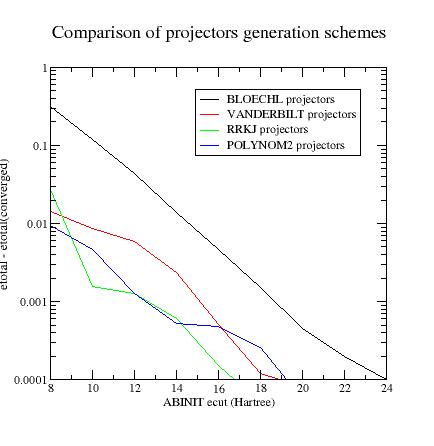
This is not a good result for a PAW dataset; let’s try to optimize it.

1^st possibility: use vanderbilt projectors instead of bloechl ones.
Vanderbilt’s projectors generally are more localized in reciprocal space than Bloechl’s ones . Keyword bloechl has to be replaced by vanderbilt in the ATOMPAW input file and $r_c$ values have to be added at the end of the file (one for each PS partial-wave). See this input file: $ABI_HOME/doc/tutorial/paw2_assets/Ni.atompaw.input.vanderbilt.

2^nd possibility: use RRKJ pseudization scheme for projectors.
Use this input file for ATOMPAW: $ABI_HOME/doc/tutorial/paw2_assets/Ni.atompaw.input2. As you can see bloechl has been changed by custom rrkj and six $r_c$ values have been added at the end of the file, each one corresponding to the matching radius of one PS partial-wave. Repeat the entire procedure (ATOMPAW + ABINIT)… and get a new ABINIT output file.
Note: You have check again log derivatives.

  ecut1     8.00000000E+00 Hartree
  ecut2     1.00000000E+01 Hartree
  ecut3     1.20000000E+01 Hartree
  ecut4     1.40000000E+01 Hartree
  ecut5     1.60000000E+01 Hartree
  ecut6     1.80000000E+01 Hartree
  ecut7     2.00000000E+01 Hartree
  ecut8     2.20000000E+01 Hartree
etotal1    -3.9599860476E+01
etotal2    -3.9626919903E+01
etotal3    -3.9627249378E+01
etotal4    -3.9627836846E+01
etotal5    -3.9628304332E+01
etotal6    -3.9628429611E+01
etotal7    -3.9628436662E+01
etotal8    -3.9628455467E+01

etotal convergence (at 1 mHartree) is achieve for $12 \le e_{cut} \le 14$ Hartree.
etotal convergence (at 0,1 mHartree) is achieve for $16 \le e_{cut} \le 18$ Hartree.

This is a reasonable result for a PAW dataset!

3^rd possibility: use enhanced polynomial pseudization scheme for projectors.
Edit Ni.atompaw.input2 and replace custom rrkj by custom polynom2 7 10. It may sometimes improve the ecut convergence.

Optional exercise¶

Let’s go back to Vanderbilt projectors.
Repeat the procedure (ATOMPAW + ABINIT) with the previous \Ni.atompaw.input.vanderbilt file.

Let’s try to change the pseudization scheme for the local pseudopotential.
Try to replace the troulliermartins keyword by ultrasoft. Repeat the procedure (ATOMPAW + ABINIT).
ABINIT can now reach convergence!

Results are below:

  ecut1     8.00000000E+00 Hartree
  ecut2     1.00000000E+01 Hartree
  ecut3     1.20000000E+01 Hartree
  ecut4     1.40000000E+01 Hartree
  ecut5     1.60000000E+01 Hartree
  ecut6     1.80000000E+01 Hartree
  ecut7     2.00000000E+01 Hartree
  ecut8     2.20000000E+01 Hartree
etotal1    -3.9608001348E+01
etotal2    -3.9613479343E+01
etotal3    -3.9616615528E+01
etotal4    -3.9620665403E+01
etotal5    -3.9622873734E+01
etotal6    -3.9623393021E+01
etotal7    -3.9623440787E+01
etotal8    -3.9623490997E+01

etotal convergence (at 1 mHartree) is achieve for $14 \le e_{cut} \le 16$ Hartree.
etotal convergence (at 0,1 mHartree) is achieve for $20 \le e_{cut} \le 22$ Hartree.

Note

You could have tried the bessel keyword instead of ultrasoft one.

Summary of convergence results

ecut convergence

Final_remarks

The localization of projectors in reciprocal space can (generally) be predicted by a look at tprod.i files. Such a file contains the curve of as a function of $q$ (reciprocal space variable). $q$ is given in $Bohr^{-1}$ units; it can be connected to ABINIT plane waves cut-off energy (in Hartree units) by: $e_{cut}=\frac{q_{cut}^2}{4}$. These quantities are only calculated for the bound states, since the Fourier transform of an extended function is not well-defined.
Generating projectors with Blochl’s scheme often gives the guaranty to have stable calculations. ATOMPAW ends without any convergence problem and DFT calculations run without any divergence (but they need high plane wave cut-off). Vanderbilt projectors (and even more custom projectors) sometimes produce instabilities during the PAW dataset generation process and/or the DFT calculations but are more efficient.
In most cases, after having changed the projector generation scheme, one has to restart the procedure from step 5.

8 Testing against physical quantities¶

The last step is to examine carefully the physical quantities obtained with our PAW dataset.

Copy $ABI_TESTS/tutorial/Input/tpaw2_2.abi in your working directory. Edit it, activate the 7 datasets (ubcomment the ‘ndtset 7` line), and use $ABI_HOME/doc/tutorial/paw2_assets/Ni.PBE-paw.rrkj.xml PAW dataset obtained from Ni.atompaw.input2 file, with a minor change of name (suppression of the indication GGA). Run ABINIT (this may take a while…).

ABINIT computes the converged ground state of ferromagnetic FCC Nickel for several volumes around equilibrium. Plot the etotal vs acell curve:

etotal vs acell

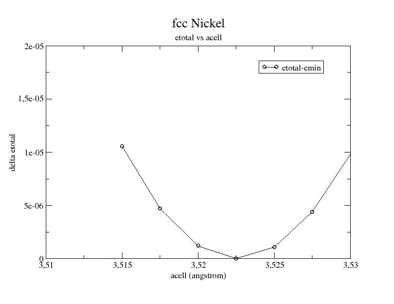
From this graph and output file, you can extract some physical quantities:

Equilibrium cell parameter:     a0 = 3.523 angstrom
Bulk modulus:                    B = 199 GPa
Magnetic moment at equilibrium: mu = 0.60

Compare these results with published results:

all-electron GGA-FLAPW from [Kresse1999]:

    a0 = 3.52 angstrom
     B = 200 GPa
    mu = 0.60

GGA-PAW with VASP code from [Kresse1999]:

    a0 = 3.52 angstrom
     B = 194 GPa
    mu = 0.61

Experimental results from from [Dewaele2008]:

    a0 = 3.52 angstrom
     B = 183 GPa

You should always compare results with all-electron ones (or other PAW computations). Not with experimental ones!

Additional remark: It can be useful to test the sensitivity of results to some ATOMPAW input parameters (see user’s guide for details on keywords):

The analytical form and the cut-off radius $r_{shape}$ of the shape function used in compensation charge density definition, By default a sinc function is used but a gaussian shape can have an influence on results. Bessel shapes are efficient and generally need a smaller cut-off radius ($r_{shape}=0.8~r_{PAW}$).
The matching radius $r_{core}$ used to generate the pseudo core density from atomic core density,
The inclusion of additional (“semi-core”) states in the set of valence electrons,
The pseudization scheme used to get pseudopotential $Vloc(r)$.

All these parameters have to be meticulously checked, especially if the PAW dataset is used for non-standard solid structures or thermodynamical domains.

Optional_exercise

Let’s add 3s and 3p semi-core states in PAW dataset!
Repeat the procedure (ATOMPAW + ABINIT) with $ABI_HOME/doc/tutorial/paw2_assets/Ni.atompaw.input.semicore file. The execution time is a bit longer as more electrons have to be treated by ABINIT.
Look at $a_0$, $B$ or $\mu$ variation.
Note: this new PAW dataset has a smaller $r_{PAW}$ radius (because semi-core states are localized).

    a0 = 3.518 angstrom
    B = 194 GPa
    mu = 0.60

9 The Real Space Optimization (RSO) - for experienced users¶

In this section, an additional optimization of the atomic data is presented. It can contribute, in some cases, to a speedup of the convergence on ecut. This optimization is not essential to produce efficient PAW datasets but can be useful.
We advise experienced users to try it.

The idea is quite simple: when expressing the different atomic radial functions ($\phi_i, \tphi_i, \tprj_i$) on the plane wave basis, the number of plane waves depends on the “locality” of these radial functions in reciprocal space.

In this paper a method to enforce the locality (in reciprocal space) of projectors $\tprj_i$ is presented; the projectors expressed in reciprocal space $\tprj_i(g)$ are modified according to the following scheme: The reciprocal space is divided in 3 regions:

If $g \lt g_{max}$, $\tprj_i(g)$ is unchanged
If $g \gt \gamma$, $\tprj_i(g)$ is set to zero
If $g_{max} \le g \le \gamma$, $\tprj_i(g)$ is modified so that the contribution of $\tprj_i(r)$ is conserved with an error $W$ (as small as possible).

RSO

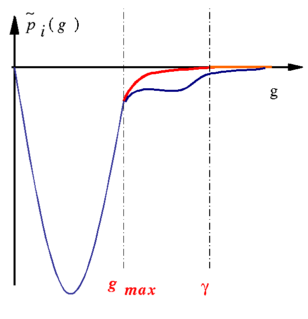
The above transformation of $\tprj_i(g)$ is only possible if $\tprj_i(r)$ is defined outside the spherical augmentation region up to a radius $R_0$, with $R_0 > r_c$. In practice we have to:

Impose an error $W$ ($W$ is the maximum error admitted on total energy)
Adjust $g_{max}$ according to $E_{cut}$ ($g_{max} \le E_{cut}$)
Choose $\gamma$ so that $2 g_{max} \lt \gamma \lt 3 g_{max}$

and let the ATOMPAW code apply the transformation to $\tprj_i$ and deduce $R_0$ radius.

You can test it now. In your working directory, use the dataset $ABI_HOME/doc/tutorial/paw2_assets/Ni.atompaw.input3 (Bloechl’s projectors).

Replace the XML options (penultimate line):

    XMLOUT
    default

with:

    XMLOUT
    rsoptim 8. 2 0.0001

8., 2 and 0.0001 are the values for $g_{max}$,$\frac{\gamma}{g_{max}}$ and $W$.

Run ATOMPAW.
You get a new PAW dataset file for ABINIT. Run ABINIT with it using the tpaw2_1.abi file.
Compare the results with those obtained in section 7.

You can try several values for $g_{max}$ (keeping $\frac{\gamma}{g_{max}}$ and $W$ constant) and compare the efficiency of the atomic data; do not forget to test physical properties again.

RSO comparison

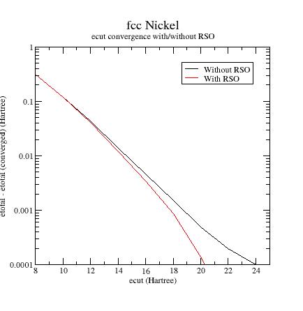
Note

How to choose the RSO parameters?
$\frac{\gamma}{g_{max}} = 2$ and $0.0001 \lt W \lt 0.001$ is a good choice. $g_{max}$ has to be adjusted. The lower $g_{max}$ the faster the convergence is but too low $g_{max}$ can produce unphysical results.