Calculation of U and J using cRPA
Using the constrained RPA to compute the U and J in the case of SrVO3.
This tutorial aims at showing how to perform a calculation of U and J in Abinit using cRPA. This method is well adapted in particular to determine U and J as they can be used in DFT+DMFT. The implementation is described in [Amadon2014].
Note that there is another methodology to compute U and J, see the Linear response U(J) tutorial.
It might be useful that you already know how to do PAW calculations using ABINIT but it is not mandatory (you can follow the two tutorials on PAW in ABINIT (PAW1, PAW2)). The DFT+U tutorial in ABINIT (DFT+U) might be useful to know some basic variables related to correlated orbitals.
The first GW tutorial in ABINIT (GW) is useful to learn how to compute the screening, and how to converge the relevant parameters (energy cutoffs and number of bands for the polarizability).
This tutorial should take two hours to complete (you should have access to more than 8 processors).
Note
Supposing you made your own installation of ABINIT, the input files to run the examples are in the ~abinit/tests/ directory where ~abinit is the absolute path of the abinit top-level directory. If you have NOT made your own install, ask your system administrator where to find the package, especially the executable and test files.
In case you work on your own PC or workstation, to make things easier, we suggest you define some handy environment variables by executing the following lines in the terminal:
export ABI_HOME=Replace_with_absolute_path_to_abinit_top_level_dir # Change this line
export PATH=$ABI_HOME/src/98_main/:$PATH      # Do not change this line: path to executable
export ABI_TESTS=$ABI_HOME/tests/             # Do not change this line: path to tests dir
export ABI_PSPDIR=$ABI_TESTS/Pspdir/  # Do not change this line: path to pseudos dir
Examples in this tutorial use these shell variables: copy and paste
the code snippets into the terminal (remember to set ABI_HOME first!) or, alternatively,
source the set_abienv.sh script located in the ~abinit directory:
source ~abinit/set_abienv.sh
The ‘export PATH’ line adds the directory containing the executables to your PATH so that you can invoke the code by simply typing abinit in the terminal instead of providing the absolute path.
To execute the tutorials, create a working directory (Work*) and
copy there the input files of the lesson.
Most of the tutorials do not rely on parallelism (except specific tutorials on parallelism). However you can run most of the tutorial examples in parallel with MPI, see the topic on parallelism.
1 The cRPA method to compute effective interaction: summary and key parameters
The cRPA method aims at computing the effective interactions among correlated electrons. Generally, these highly correlated materials contain rare-earth metals or transition metals, which have partially filled d or f bands and thus localized electrons. cRPA relies on the fact that screening processes can be decomposed in two steps: Firstly, the bare Coulomb interaction is screened by non correlated electrons to produce the effective interaction Wr.
Secondly, correlated electrons screened this interaction to produce the fully screening interaction W [Aryasetiawan2004]). However, the second screening process is taken into account when one uses a method which describes accurately the interaction among correlated electrons (such as Quantum Monte Carlo within the DFT+DMFT method). So, to avoid a double counting of screening by correlated electrons, the DFT+DMFT methods needs as an input the effective interaction Wr. The goal of this tutorial is to present the implementation of this method using Projected Local Orbitals Wannier orbitals in ABINIT (The implementation of cRPA in ABINIT is described in [Amadon2014] and projected local orbitals Wannier functions are presented in [Amadon2008]). The discussion about the localization of Wannier orbitals has some similarities with the beginning of the DMFT tutorial (see here and there
Several parameters (both physical and technical) are important for the cRPA calculation:
-
The definition of correlated orbitals. The first part of the tutorial is similar to the DMFT tutorial but uses different keywords to calculate the correlated orbitals basis. It explains the electronic structure of SrVO3 and will be used to understand the definition of Wannier orbitals with various extensions. Wannier functions are unitarily related to a selected set of Kohn Sham (KS) wavefunctions, specified in ABINIT by band index plowan_bandi, and plowan_bandf. As empty bands are necessary to build Wannier functions, it is required in DMFT or cRPA calculations that the KS Hamiltonian is correctly diagonalized: use high values for nnsclo, and nline for cRPA and DMFT calculations and preceding DFT calculations. Another solution used in the present tutorial is to use a specific non self-consistent calculation to diagonalize the hamiltonian, as in GW calculations. Concerning the localization or correlated orbitals, generally, the larger plowan_bandf-plowan_bandi is, the more localized is the radial part of the Wannier orbital. Finally, note that Wannier orbitals are used in DMFT and cRPA implementations but this is not the most usual choice of correlated orbitals in the DFT+U implementation in particular in ABINIT (see [Amadon2008a]). The relation between the two expressions is briefly discussed in [Geneste2017].
-
The constrained polarization calculation. As we will discuss in section 2, there are different ways to define the constrained polarizability, by suppressing in the polarization, some electronic transitions: As discussed in section I of [Amadon2014], one can either suppress electronic transition inside a given subset of Kohn-Sham bands. In this case, one can use ucrpa=1, and choose the first and last bands defining the subset of bands by using variable ucrpa_bands. One can also use an energy windows instead of a number of bands by using ucrpa_window. Another solution is to use a weighting scheme which lowers the contribution of a given transition, as a function of the weight of correlated orbitals on the bands involved in the transition (see Eq. (5) and (7) in [Amadon2014]). In this case, on still use the variable ucrpa_bands. The variable will in this case be used to define Projected Local Orbitals Wannier functions that will then be used to define the weighting function in the polarizability. (see Eq. (5) and (7) in [Amadon2014]).
-
Convergence parameters are the same as for a polarizability calculation for the screening calculation (ecuteps, ecutwfn, nband) and the same as for the exchange part of GW for the effective interaction, ie ecutsigx, ecutwfn. It is recommended, as discussed in appendix A of [Amadon2014], to use pawoptosc=1. If the calculation is carried out with several atoms, use nsym=1, the calculation is not symmetrized over atoms in this case.
2 Electronic Structure of SrVO3 in LDA
Before continuing, you might consider to work in a different subdirectory as
for the other tutorials. Why not Work_crpa?
In what follows, the name of files are mentioned as if you were in this subdirectory.
All the input files can be found in the $ABI_TESTS/tutoparal/Input directory.
Copy the files tucalc_crpa_1.abi from ABI_TESTS/tutoparal/Input to Work_crpa with:
cd $ABI_TESTS/tutoparal/Input
mkdir Work_crpa
cd Work_crpa
cp ../tucalc_crpa_1.abi .
and run the code with:
mpirun -n 32 abinit tucalc_crpa_1.abi > log_1 &
This run should take some time. It is recommended that you use at least 10 processors (and 32 should be fast). It calculates the LDA ground state of SrVO3 and compute the band structure in a second step. The variable pawfatbnd allows to create files with “fatbands” (see description of the variable in the list of variables): the width of the line along each k-point path and for each band is proportional to the contribution of a given atomic orbital on this particular Kohn Sham Wavefunction. A low cutoff and a small number of k-points are used in order to speed up the calculation. During this time you can take a look at the input file.
There are two datasets. The first one is a ground state calculations with nnsclo=3 and nline=3 in order to have well diagonalized eigenfunctions even for empty states. In practice, you have however to check that the residue of wavefunctions is small at the end of the calculation. In this calculation, we find 1.E-06, which is large (1.E-10 would be better, so nline and nnsclo should be increased, but it would take more time). When the calculation is finished, you can plot the fatbands for Vanadium and l=2 with
xmgrace tucalc_crpa_O_DS2_FATBANDS_at0001_V_is1_l0002 -par ../Input/tdmft_fatband.par
The band structure is given in eV.
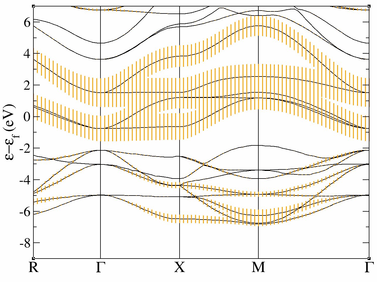
and the fatbands for all Oxygen atoms and l=1 with
xmgrace tucalc_crpa_O_DS2_FATBANDS_at0003_O_is1_l0001 tucalc_crpa_O_DS2_FATBANDS_at0004_O_is1_l0001 tucalc_crpa_O_DS2_FATBANDS_at0005_O_is1_l0001 -par ../Input/tdmft_fatband.par
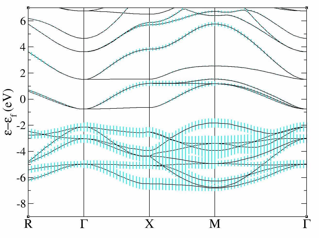
In these plots, you recover the band structure of SrVO3 (see for comparison the band structure of Fig.3 of [Amadon2008]), and the main character of the bands. Bands 21 to 25 are mainly d and bands 12 to 20 are mainly oxygen p. However, we clearly see an important hybridization. The Fermi level (at 0 eV) is in the middle of bands 21-23.
One can easily check that bands 21-23 are mainly d-t2g and bands 24-25 are mainly eg: just use pawfatbnd = 2 in tucalc_crpa_1.abi and relaunch the calculations. Then the file tucalc_crpa_O_DS2_FATBANDS_at0001_V_is1_l2_m-2, tucalc_crpa_O_DS2_FATBANDS_at0001_V_is1_l2_m-1 and tucalc_crpa_O_DS2_FATBANDS_at0001_V_is1_l2_m1 give you respectively the xy, yz and xz fatbands (ie d-t2g) and tucalc_crpa_O_DS2_FATBANDS_at0001_V_is1_l2_m+0 and tucalc_crpa_O_DS2_FATBANDS_at0001_V_is1_l2_m+2 give the z2 and x2-y2 fatbands (ie eg).
So in conclusion of this study, the Kohn Sham bands which are mainly t2g are the bands 21, 22 and 23.
Of course, it could have been anticipated from classical crystal field theory: the vanadium is in the center of an octahedron of oxygen atoms, so d orbitals are split in t2g and eg. As t2g orbitals are not directed toward oxygen atoms, t2g-like bands are lower in energy and filled with one electron, whereas eg-like bands are higher and empty.
In the next section, we will thus use the d -like bands to built Wannier functions and compute effective interactions for these orbitals.
3 Definition of screening and orbitals in cRPA: models, input file and log file
3.1. The constrained polarization calculation.
As discussed briefly in Appendix A of [Amadon2014] as well as in section III B of [Vaugier2012] and Section II B of [Sakuma2013], one can use different schemes for the cRPA calculations. Let us discuss these different models namely the ( d-d ), ( dp-dp ), ( d-dp (a)), and ( d-dp (b)) models. In the notation (A-B), A and B refers respectively to some bands of A-like and B-like character. Moreover, A refers to the definition of screening and B refers to the definition of correlated orbitals. To clarify this definition, we give below some examples:
- ( t2g-t2g) model (or t2g model): The correlated orbitals are defined with only t2g-like bands (bands 21, 22 and 23). The screening inside these bands is not taken into account to built the constrained polarizability. Note that if this case (and in the ( d-d ) and ( dp-dp ) models), using ucrpa=1 or 2 give the same results, provided one uses ucrpa_bands equal to (plowan_bandi plowan_bandf ).
- ( d-d ) model (or d model): The correlated orbitals are defined with only d -like bands (bands 21 to 25). The screening inside these bands is not taken into account.
- ( dp-dp ) model (or dp model): The correlated orbitals are defined with only d -like and Op-like bands (bands 12 to 23). The screening inside these bands is not taken into account.
- ( d-dp (a)) model: In this scheme the Wannier orbitals are constructed as in the ( dp-dp ) model. However, in this scheme, one only supresses the screening inside d -like bands (ucrpa=1). It is coherent with the fact that the DMFT will only be applied to the d orbitals: so the screening for Op-like bands need to be taken into account.
- ( d-dp (b)) model: It is the same model as the ( d-dp (a)), nevertheless, in this case, only the weighting scheme is used (ucrpa=2 in ABINIT). Which way of computing interactions is the most relevant depends on the way the interactions will be used. Some aspects of it are discussed in Ref. [Vaugier2012]. Also, for Mott insulators, and if self-consistency over interactions is carried out, the choice of models is discussed in [Amadon2014].
3.2. The input file for cRPA calculation: correlated orbitals, Wannier functions
In this section, we will present the input variables and discuss how to extract useful information in the log file in the case of the d-d model. The input file for a typical cRPA calculation (tucalc_crpa_2.abi) contains four datasets (as usual GW calculations, see the GW tutorial): the first one is a well converged LDA calculation, the second is non self-consistent calculation to compute accurately full and empty states, the third computes the constrained non interacting polarizability, and the fourth computes effective interaction parameters U and J. We discuss these four datasets in the next four subsections.
Copy the file in your Work_crpa directory with:
cp ../tucalc_crpa_2.abi .
The input file tucalc_crpa_2.abi contains standard data to perform a LDA calculation on SrVO3. We focus in the next subsections on some peculiar input variables related to the fact that we perform a cRPA calculation. Before reading the following section, launch the abinit calculation:
abinit tucalc_crpa_2.abi > log_2
3.2.1. The first DATASET: A converged LDA calculation
The first dataset is a simple calculation of the density using LDA using 50 bands. We do not use symmetry in this calculation, so nsym=1. If symmetry is used (nsym=0), then the calculation of U and J will be valid, but the full interaction matrix described in section 3.2.4 will not be correct.
3.2.2. The second DATASET: A converged LDA calculation and definition of Wannier functions
Before presenting the input variables for this dataset, we discuss two important physical parameters relevant to this dataset.
-
Diagonalization of Kohn-Sham Hamiltonian: As in the case of DFT+DMFT or GW calculation, a cRPA calculation requires that the LDA is perfectly converged and the Kohn Sham eigenstates are precisely determined, including the empty states. Indeed these empty states are necessary both to build Wannier functions and to compute the polarizability. For this reason we choose a very low value of tolwfr in the input file tucalc_crpa_1.abi.
-
Wannier functions: Once the calculation is converged, we compute Wannier functions, triggered using the plowan_compute keyword. In addition to the KS bands (defined using plowan_bandi and plowan_bandf), we use the (PLO-Wannier) keywords to define on which atom and on which orbital the Wannier functions are calculated.
For this tutorial we will only look at cases with only one orbital for the Wannier functions and thus the cRPA, but note that the implementation allow to use multiple orbitals. We emphasize that with respect to the discussion on models on section 3.1, plowan_bandi and plowan_bandf are used to define the so called A bands. We will see in dataset 2 how B bands are defined. In our case, as we are in the d-d model, we choose only the d -like bands as a starting point and plowan_bandi and plowan_bandf are thus equal to the first and last d -like bands, namely 21 and 25.
    getden2        -1
    # == Compute empty bands precisely
    iscf2          -2
    tolwfr2   1.0d-18     # Will stop when this tolerance is achieved

    # == Compute Projected Wannier functions
    plowan_compute2 1 # Activate the computation of Wannier functions
    plowan_bandi 21 # First band for Wannier functions
    plowan_bandf 25 # Last band for Wannier functions
    plowan_natom 1 # Number of atoms
    plowan_iatom 1  # Index of atoms
    plowan_nbl 1  # Number of orbitals on each atoms
    plowan_lcalc 2  # Index of the orbitals (2 -> d)
    plowan_projcalc 5  # Projector for the orbitals (see pseudo-potential file)
3.2.2. The third DATASET: Compute the constrained polarizability and dielectric function
The third DATASET drives the computation of the constrained polarizability and the dielectric function. Again, we reproduce below the input variables peculiar to this dataset.
We add some comments here on three most important topics
- Definition of constrained polarizability: As in the discussion on models on section 3.1, the constrained polarizability is defined thanks to B-like bands. The keywords related to this definition is ucrpa_bands. According to the value of ucrpa, ucrpa_bands defined the bands for which the transitions are neglected, or (if ucrpa=2), it defined Wannier functions that are used in the weighting scheme (see Eq. (5) and (7) of section II of [Amadon2014]). Alternatively and only if ucrpa=1, an energy windows can be defined (with variable ucrpa_window) to exclude the transition. In our case, as we are in the d-d model, we neglect transitions inside the d -like bands, so we choose ucrpa_bands= 21 25.
- Reading of the Wannier functions : plowan_compute defined to 10 reads the Wannier functions in file ‘’data.plowann’‘.
- Convergence of the polarizability: nband and ecuteps are the two main variables that should be converged. Note that one must study the role of these variables directly on the effective interaction parameters to determine their relevant values.
- Frequency mesh of the polarizability: Can be useful if one wants to plot the frequency dependence of the effective interactions (as in e.g. [Amadon2014]).
optdriver3     3     # Keyword to launch the calculation of screening
gwcalctyp3     2     # The screening will be used later with gwcalctyp 2
                     # in the next dataset
getwfk3       -1     # Obtain WFK file from previous dataset
ecuteps3     5.0     # Cut-off energy of the planewave set to represent
                     #   the dielectric matrix.
                     # It is important to converge effective interactions
                     #   as a function of this parameter.

# -- Frequencies for dielectric matrix
nfreqre3       1     # Number of  real frequencies
freqremax3    10 eV  # Maximal value of frequencies
freqremin3     0 eV  # Minimal value of frequencies
nfreqim3       0     # Number of  imaginary frequencies

# -- Ucrpa: screening
ucrpa_bands3  21 25  # Define the bands corresponding to the _d_ contribution

plowan_compute3 10 # Read Wannier functions

# -- Parallelism
gwpara3        1
3.2.3. The fourth DATASET: Compute the effective interactions
The fourth DATASET drives the computation of the effective interactions. It is similar computationally to the computation of exchange in GW calculations. Again, we reproduce below the input variables peculiar to this dataset.
We add some comments on convergence properties
-
Convergence as the number of plane waves: Eq. (A1) and (A2) in Appendix A of [Amadon2014] show the summation over plane waves which is performed. The cutoff on plane wave which is used in this summation is ecutsigx because of the similarity of Eq. A2 with the Fock exchange (see GW notes when one computes the bare interaction. ecutsigx is thus the main convergence parameter for this dataset. Note that as discussed in Appendix A of [Amadon2014], high values of ecutsigx can be necessary because oscillator matrix elements in PAW contains the Fourier transform of (a product of) atomic orbitals.
-
The frequency mesh must be the same as in the DATASET 2.
     optdriver4  4      # Self-Energy calculation
     gwcalctyp4  2      # activate HF or ucrpa
     getwfk4     1      # Obtain WFK file from dataset 1
     getscr4     2      # Obtain SCR file from previous dataset
     ecutsigx4  30.0    # Dimension of the G sum in Sigma_x.
     plowan_compute4 10 # Read Wannier functions
     # -- Frequencies for effective interactions
     nfreqsp4    1
     freqspmax4 10 eV
     freqspmin4  0 eV
     nkptgw4     0      # number of k-point where to calculate
                        # the GW correction: all BZ is used
     mqgrid4   300      # Reduced but fine at least for SrVO3
     mqgriddg4 300      # Reduced but fine at least for SrVO3

     # -- Parallelism
     gwpara4 2          # do not change if nsppol=2
3.2.4 The cRPA calculation: the log file (for the d-d model)
We are now going to browse quickly the log file for this calculation.
- Bare interaction of atomic orbitals.
First, at the beginning of the log file, you will find the calculation of the bare interaction for the atomic wavefunction corresponding the angular momentum specified by lpawu, in the input file (here lpawu =2). It is a simple fast direct integration. Note that this information is complete only if you use XML PAW atomic data (as the one available on the JTH table available on the ABINIT website).
      =======================================================================
      == Calculation of diagonal bare Coulomb interaction on ATOMIC orbitals
         (it is assumed that the wavefunction for the first reference
                 energy in PAW atomic data is an atomic eigenvalue)

     Max value of the radius in atomic data file   =    201.3994
     Max value of the mesh   in atomic data file   =    910
     PAW radius is                                 =      2.2000
     PAW value of the mesh for integration is      =    587
     Integral of atomic wavefunction until rpaw    =      0.8418

     For an atomic wfn truncated at rmax =    201.3994
         The norm of the wfn is                    =      1.0000
         The bare interaction (no renormalization) =     17.7996 eV
         The bare interaction (for a renorm. wfn ) =     17.7996 eV

     For an atomic wfn truncated at rmax =      2.2000
         The norm of the wfn is                    =      0.8418
         The bare interaction (no renormalization) =     16.0038 eV
         The bare interaction (for a renorm. wfn ) =     22.5848 eV
     =======================================================================
Various quantities are computed, the one which is interesting to see here, is the bare interaction computed for a wavefunction truncated at a very large radius (here 201.3994 au ), ie virtually infinite. We find that this bare interaction is 17.8 eV. We will compare below this value to the bare interaction computed on Wannier orbitals.
- Bare Coulomb direct interaction of Wannier orbitals. In the third dataset, the code writes the Coulomb interaction matrix as:
          U'=U(m1,m2,m1,m2) for the bare interaction
     -      1      2      3      4      5
       1 16.041 14.898 14.885 14.898 15.715
       2 14.898 16.041 15.508 14.898 15.092
       3 14.885 15.508 16.567 15.508 15.114
       4 14.898 14.898 15.508 16.041 15.092
       5 15.715 15.092 15.114 15.092 16.567
- First we see that diagonal interactions are larger than off-diagonal terms, which is logical, because electron interaction is larger if electrons are located in the same orbital.
- We recover in this interaction matrix the degeneracy of d orbitals in the cubic symmetry (we remind, as listed in dmatpawu, that the order of orbitals in ABINIT are xy, yz, z2, xy, x2-y2).
- We note also that the interaction for t2g and eg orbitals are not the same. This effect is compared in e.g. Appendix C.1 of [Vaugier2012] to the usual Slater parametrization of interaction matrices.
- Diagonal bare interactions are smaller to the bare interaction on atomic orbitals (17.8 eV, as discussed above). It shows that the Wannier functions (obtained within the d-d model) are less localized than atomic orbitals. It is logical because these Wannier functions contain indeed a weight on O- p orbitals.
- From this interaction matrix, one can compute the average of all elements (the famous U ), as well as the average of diagonal elements, which is sometimes used as another definition of U (see Eq. (8) and (9) of [Amadon2014]. The two quantities are written in the log file:
    Hubbard bare interaction U=1/(2l+1)**2 \sum U(m1,m2,m1,m2)=   15.3789    0.0000

(Hubbard bare interaction U=1/(2l+1) \sum U(m1,m1,m1,m1)=   16.2514    0.0000)
Important
To speed up the calculation and if one needs only these average values of U and J, one can use nsym = 0 in the input file, but in this case, the interaction matrix does not anymore reproduce the correct symmetry. For several correlated atoms, the implementation is under test and it is mandatory to use nsym=1.]
- Bare exchange interaction. The exchange interaction matrix is also written as well as the average of off-diagonal elements, which is J.
       Hund coupling J=U(m1,m1,m2,m2) for the bare interaction
         1      2      3      4      5
    1 16.041  0.482  0.555  0.478  0.249
    2  0.482 16.041  0.329  0.478  0.478
    3  0.555  0.329 16.567  0.400  0.555
    4  0.478  0.478  0.400 16.041  0.482
    5  0.249  0.478  0.555  0.482 16.567

    bare interaction value of J=U-1/((2l+1)(2l)) \sum_{m1,m2} (U(m1,m2,m1,m2)-U(m1,m1,m2,m2))=    0.6667    0.0000
- Then, the cRPA effective interactions are given for all frequencies. The first frequency is zero and the cRPA interactions are:
     U'=U(m1,m2,m1,m2) for the cRPA interaction
       1      2      3      4      5
  1  3.434  2.432  2.338  2.432  2.966
  2  2.432  3.434  2.809  2.432  2.495
  3  2.338  2.809  3.641  2.809  2.430
  4  2.432  2.432  2.809  3.434  2.495
  5  2.966  2.495  2.430  2.495  3.641

 Hubbard cRPA interaction for w =  1, U=1/(2l+1)**2 \sum U(m1,m2,m1,m2)=    2.7546   -0.0000

 (Hubbard cRPA interaction for w =   1, U=1/(2l+1) \sum U(m1,m1,m1,m1)=    3.5167   -0.0000)

 Hund coupling J=U(m1,m1,m2,m2) for the cRPA interaction
       1      2      3      4      5
  1  3.434  0.440  0.508  0.435  0.247
  2  0.440  3.434  0.315  0.436  0.442
  3  0.508  0.315  3.641  0.378  0.444
  4  0.435  0.436  0.378  3.434  0.446
  5  0.247  0.442  0.444  0.446  3.641

  cRPA interaction value of J=U-1/((2l+1)(2l)) \sum_{m1,m2} (U(m1,m2,m1,m2)-U(m1,m2,m2,m1))=    0.5997    0.0000
- At the end of the calculation, the value of U and J as a function of frequency are gathered.
       -------------------------------------------------------------
                Average U and J as a function of frequency
       -------------------------------------------------------------
             omega           U(omega)            J(omega)
            0.000      2.7546   -0.0000      0.5997    0.0000
       -------------------------------------------------------------
4 Convergence studies
We give here the results of some convergence studies, than can be made by the readers. Some are computationally expensive. It is recommanded to use at least 32 processors. Input file is provided in tucalc_crpa_3.abi for the first case.
4.1 Cutoff in energy for the polarisability ecuteps
The number of plane waves used in the calculation of the cRPA polarizability is determined by ecuteps (see Notes on RPA calculations). The convergence can be studied simply by increasing the values of ecuteps and gives:
So, for nband=30, ecutsigx=30 and a 4x4x4 k-point grid, the effective interactions are converged with a precision of 0.02 eV for ecuteps=5.
4.2 Number of bands nband
The RPA polarizability depends also of the number of Kohn-Sham bands as also discussed in the Notes on RPA calculations)
So, for ecuteps=5, ecutsigx=30 and a 4x4x4 k-point grid, the effective interactions are converged with a precision of 0.05 eV for nband=50.
4.3 Cutoff in energy for the calculation of the Coulomb interaction ecutsigx
ecutsigx is the input variable determining the number of plane waves used in the calculation of the exchange part of the self-energy. The same variable is used here to determine the number of plane waves used in the calculation of the effective interaction. The study of the convergence gives:
For ecuteps=3, nband=30 and a 4 4 4 k-point grid, effective interactions are converged with a precision of 0.02 eV for ecutsigx=30 Ha.
4.4 k-point
The dependence of effective interactions with the k-point grid is also important to check.
For ecuteps=3, nband=30 and ecutsigx=30, effective interactions are converged to 0.01 eV for a k-point grid of 6 6 6. The converged parameters are thus ecuteps=5,ecutsigx=30,ngkpt=6 6 6, nband=50 with an expected precision of 0.1 eV. We will use instead ecuteps=5,ecutsigx=30,ngkpt=4 4 4, nband=50 to lower the computational cost. In this case, we find values of U and J of 2.75 eV and 0.41 eV and U is probably underestimated by 0.1 eV.
5 Effective interactions for different models
In this section, we compute, using the converged values of parameters, the value of effective interactions for the models discussed in section and 3.1. The table below gives for each model, the values of plowan_bandi, plowan_bandf and ucrpa_bands that must be used, and it sums up the value of bare and effective interactions.
Even if our calculation is not perfectly converged with respect to k-points, the results obtained for the d-d, dp-dp, and d-dp (a) models are in agreement (within 0.1 or 0.2 eV) with results obtained in Table V of [Amadon2014] and references cited in this table.
To obtain the results with only the t2g orbitals, one must use a specific input file, which is tucalc_crpa_4.abi, which uses specific keywords, peculiar to this case (compare it with tucalc_crpa_2.abi). In this peculiar case, the most common definition of J has to be deduced by direct calculation from the interaction matrices using the Slater Kanamori expression (see e.g. [Lechermann2006] or [Vaugier2012]) and not using the value of J computed in the code).
We now briefly comment the physics of the results.
-
Bare interactions. When the number of bands used is larger, the Wannier orbitals extension is smaller. Thus, the interaction obtained with Wannier functions obtained from dp bands are larger than interactions obtained with Wannier functions obtained with d bands and also larger than interaction obtained on atomic orbitals.
-
For the same Wannier functions ( dp-dp, d-dp (a), d-dp (b)), one can see the role of the screening on cRPA interactions:
- When one supresses all transitions inside the d -like and p -like bands ( dp-dp model), U is large.
- When only the transitions inside the d -like bands are suppressed, U is smaller ( d-dp (a) model) in comparison to the dp-dp model, because the screening is more efficient.
- Lastly, when one uses the weighting scheme to compute the polarizability, U is very small. Indeed, in this case, one can show that there are some residual transitions near the Fermi level (due to the hybridization between d orbitals and O p orbitals) which are very efficient to screen the interaction (A similar effect is discussed in [Amadon2014] for UO 2 or [Sakuma2013] for transition metal oxydes).
Finally, fully screened interactions (not discussed here) could also be computed for each definition of correlated orbitals by using the default values of ucrpa_bands.
6 Frequency dependent interactions
In this section, we are going to compute frequency dependent effective interactions. Just change the following input variables in order to compute effective interaction between 0 and 30 eV. We use nsym = 0 in order to decrease the computational cost.
 # -- Frequencies for effective interactions
 nsym        0
 nfreqsp3   60
 freqspmax3 30 eV
 freqspmin3  0 eV
 nfreqsp4   60
 freqspmax4 30 eV
 freqspmin4  0 eV
An example of input file can be found in tucalc_crpa_5.abi. Note that we have decreased some parameters to speed-up the calculations. Importantly, however, we have increased the number of Kohn Sham bands, because calculation of screening at high frequency involves high energy transitions which requires high energy states (as well as semicore states). If the calculation is too time consuming, you can reduce the number of frequencies. The following figure has been plotted with 300 frequencies, but using 30 or 60 frequencies is sufficient to see the main tendencies. Extract the value of U for the 60 frequencies using:
grep "U(omega)" -A 60 tucalc_crpa_5.out > Ufreq.dat
Remove the first line, and plot the data:
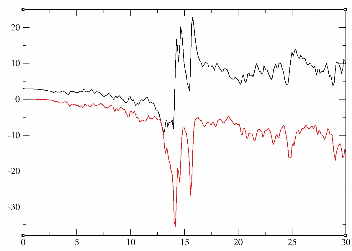
We recover in the picture the main results found in the Fig. 3 of [Aryasetiawan2006]. Indeed, the frequency dependent effective interactions exhibits a plasmon excitation.
7 Conclusion
This tutorial showed how to compute effective interactions for SrVO3. It emphasized the importance of the definition of correlated orbitals and the definition of constrained polarizability.