Second tutorial on DFPT:
Phonon band structures, thermodynamical properties.
In this tutorial you will learn how to post-process the raw data of the Abinit DFPT calculations to get the following physical properties of periodic solids:
- Interatomic forces constants
- Phonon band structures
- Thermodynamical properties
Visualisation tools are NOT covered in this tutorial. Powerful visualisation procedures have been developed in the Abipy context, relying on matplotlib. See the README of Abipy and the Abipy tutorials.
This tutorial should take about 1 hour.
WARNING : This tutorial has been updated by removing the use of the ANADDB input variable brav in trf2_4.abi, trf2_5.abi, and trf2_6.abi, with the accompanying modifications in the text of the tutorial. Also, due to the change of default values for rfdir and rfatpol in ABINITv9.8 with respect to the prior versions of ABINIT, the example input files from this tutorial will not work with such version of ABINIT or even older ones). Please, use ABINITv9.8 or more recent versions of ABINIT, or adjust the values of rfdir and rfatpol. See point A.3 of the v9.8 release notes.
Note
Supposing you made your own installation of ABINIT, the input files to run the examples are in the ~abinit/tests/ directory where ~abinit is the absolute path of the abinit top-level directory. If you have NOT made your own install, ask your system administrator where to find the package, especially the executable and test files.
In case you work on your own PC or workstation, to make things easier, we suggest you define some handy environment variables by executing the following lines in the terminal:
export ABI_HOME=Replace_with_absolute_path_to_abinit_top_level_dir # Change this line
export PATH=$ABI_HOME/src/98_main/:$PATH      # Do not change this line: path to executable
export ABI_TESTS=$ABI_HOME/tests/             # Do not change this line: path to tests dir
export ABI_PSPDIR=$ABI_TESTS/Pspdir/  # Do not change this line: path to pseudos dir
Examples in this tutorial use these shell variables: copy and paste
the code snippets into the terminal (remember to set ABI_HOME first!) or, alternatively,
source the set_abienv.sh script located in the ~abinit directory:
source ~abinit/set_abienv.sh
The ‘export PATH’ line adds the directory containing the executables to your PATH so that you can invoke the code by simply typing abinit in the terminal instead of providing the absolute path.
To execute the tutorials, create a working directory (Work*) and
copy there the input files of the lesson.
Most of the tutorials do not rely on parallelism (except specific tutorials on parallelism). However you can run most of the tutorial examples in parallel with MPI, see the topic on parallelism.
0 Generation of necessary input wavefunctions
Before beginning, you might consider working in a different subdirectory as for the other tutorials, in order to help keep track of all the files. Why not create Work_rf2 in $ABI_TESTS/tutorespfn/Input?
As the DFPT equations at higher order always start from input wavefunctions obtained at lower order, we begin by generating the ground state wavefunctions and DDK wavefunctions for our system, AlAs. The ground state wavefunctions are needed for the phonon and electric field perturbations, and the electric field perturbation needs the DDK wavefunctions as well, as explained in the first tutorial on DFPT.
Copy file trf2_1.abi from $ABI_TESTS/tutorespfn/Input* to Work_rf2:
cd $ABI_TESTS/tutorespfn/Input;
mkdir Work_rf2;
cd Work_rf2;
cp ../trf2_1.abi
abinit trf2_1.abi >& log &
Let us have a look at the input file trf2_1.abi.
# Crystalline AlAs : computation of the phonon spectrum

# initial steps: compute ground state wavefunctions accurately and the DDK
# wavefunctions accurately

  ndtset 2

# first dataset: accurate ground state wavefunctions
  kptopt1  1            # Automatic generation of k points, taking
                        # into account all symmetries
  tolvrs1   1.0d-18     # SCF stopping criterion

# second dataset: DDK wavefunctions, needed later for electric field
  kptopt2 2             # DDK can use only time reveral symmetry
  getwfk2 -1            # require ground state wavefunctions from previous run
  rfelfd2 2             # activate DDK perturbation
  iscf2   -3            # this is a non-self-consistent calculation
  tolwfr2 1.0D-20       # tight convergence on wavefunction residuals

#######################################################################
#Common input variables

#Definition of the unit cell
    acell   3*10.61         # This is equivalent to   10.61 10.61 10.61
    rprim   0.0  0.5  0.5   # In tutorials 1 and 2, these primitive vectors
            0.5  0.0  0.5   # (to be scaled by acell) were 1 0 0  0 1 0  0 0 1
            0.5  0.5  0.0   # that is, the default.

#Definition of the atom types
   ntypat   2         # There are two types of atom
    znucl   13 33     # The keyword "znucl" refers to the atomic number of the
                      # possible type(s) of atom. The pseudopotential(s)
                      # mentioned in the "files" file must correspond
                      # to the type(s) of atom. Here, type 1 is the Aluminum,
                      # type 2 is the Arsenic.

#Definition of the atoms
    natom   2         # There are two atoms
    typat   1 2       # The first is of type 1 (Al), the second is of type 2 (As).

     xred   0.0  0.0  0.0
            0.25 0.25 0.25

#Gives the number of band, explicitly (do not take the default)
    nband   4

#Definition of the planewave basis set
     ecut   3.0           # Maximal kinetic energy cut-off, in Hartree

#Definition of the k-point grid
    ngkpt   4  4  4
  nshiftk   4              # Use one copy of grid only (default)
   shiftk   0.0 0.0 0.5    # This gives the usual fcc Monkhorst-Pack grid
            0.0 0.5 0.0
            0.5 0.0 0.0
            0.5 0.5 0.5

#Definition of the SCF procedure
    nstep   25         # Maximal number of SCF cycles
   diemac   9.0        # Although this is not mandatory, it is worth to
                       # precondition the SCF cycle. The model dielectric
                       # function used as the standard preconditioner
                       # is described in the "dielng" input variable section.
                       # The dielectric constant of AlAs is smaller that the one of Si (=12).


pp_dirpath "$ABI_PSPDIR"
pseudos "13al.981214.fhi, PseudosTM_pwteter/33as.pspnc"

##############################################################
# This section is used only for regression testing of ABINIT #
##############################################################
#%%<BEGIN TEST_INFO>
#%% [setup]
#%% executable = abinit
#%% test_chain = trf2_1.abi, trf2_2.abi, trf2_3.abi, trf2_4.abi, trf2_5.abi, trf2_6.abi
#%% [shell]
#%% post_commands = ww_cp trf2_1o_DS1_WFK trf2_2o_DS99_WFK; ww_cp trf2_1o_DS2_1WF7 trf2_2o_DS98_1WF7; ww_cp trf2_1o_DS2_1WF8 trf2_2o_DS98_1WF8; ww_cp trf2_1o_DS2_1WF9 trf2_2o_DS98_1WF9;
#%% [files]
#%% files_to_test =
#%%   trf2_1.abo, tolnlines= 0, tolabs=  0.000e+00, tolrel=  0.000e+00
#%% [paral_info]
#%% max_nprocs = 2
#%% [extra_info]
#%% authors = X. Gonze, J. Zwanziger
#%% keywords = NC, DFPT
#%% description =  Crystalline AlAs : computation of the phonon spectrum
#%%<END TEST_INFO>
This input file consists of two datasets–the first generates the
ground state wavefunctions, with tight convergence: these are output
in the file trf2_1o_DS1_WFK. The second dataset uses these
wavefunctions to generate the DDK wavefunctions, which are output in
the files trf2_1o_DS2_1WF7, trf2_1o_DS2_1WF8, and
trf2_1o_DS2_1WF9. Depending on the details of your build, these
files might be appended with .nc, if they are produced in netcdf
format.
A note on the naming convention–the DDK files here are named 1WF7, 1WF8, and 1WF9. The “1” signifies a first-order wavefunction. Then, ABINIT numbers each perturbation, such that the phonons are numbered 1…3N, for an N atom system. Here N = 2 for AlAs. The DDK perturbations are numbered 3N+1, 3N+2, and 3N+3, for the three cartesian directions, giving in this case 7, 8, and 9.
1 Generation of a derivative database
With the necessary input wavefunctions generated, we are ready to compute the derivative database.
Copy the file trf2_2.abi from $ABI_TESTS/tutorespfn/Input* into your working directory:
cp ../trf2_2.abi .
Examine the input file you are about to run:
# Crystalline AlAs : computation of the phonon spectrum and electric field perturbation

   ndtset   8

#Q vectors for all datasets

#Complete set of symmetry-inequivalent qpt chosen to be commensurate
# with kpt mesh so that only one set of GS wave functions is needed.

   nqpt   1            # One qpt for each dataset (only 0 or 1 allowed)
   qptopt 1            # activate determining qpts in IBZ with symmetry
   ngqpt  4 4 4        # these variables mirror those used for the kpt
   nshiftq 1           # mesh below, but with no shift. In this way,
   shiftq 0 0 0        # qpts coherent with the kpts are constructed
                       # the number of resulting q pts is pretdetermined
                       # through use of the abitk tool

   iqpt: 1 iqpt+ 1     # we automatically iterate through the q pts


#Set 1 : iqpt 1 is the gamma point, so Q=0 phonons and electric field pert.

  getddk1   98         # d/dk wave functions
  kptopt1   2          # Modify default to use time-reversal symmetry
  rfelfd1   3          # Electric-field perturbation response
                       # (in addition to default phonon)

#Sets 2-8 : Finite-wave-vector phonon calculations (defaults for all datasets)

   getwfk   99         # Use GS wave functions
   kptopt   3          # Need full k-point set for finite-Q response
   rfphon   1          # Do phonon response
   tolvrs   1.0d-8     # Converge on potential residual

# turn off various file outputs, here we will be interested only the
# DDB files

   prtwf 0
   prtden 0
   prtpot 0
   prteig 0

#######################################################################
#Common input variables

#Definition of the unit cell
    acell   3*10.61         # This is equivalent to   10.61 10.61 10.61
    rprim   0.0  0.5  0.5   # In tutorials 1 and 2, these primitive vectors
            0.5  0.0  0.5   # (to be scaled by acell) were 1 0 0  0 1 0  0 0 1
            0.5  0.5  0.0   # that is, the default.

#Definition of the atom types
   ntypat   2         # There are two types of atom
    znucl   13 33     # The keyword "znucl" refers to the atomic number of the
                      # possible type(s) of atom. The pseudopotential(s)
                      # mentioned in the "files" file must correspond
                      # to the type(s) of atom. Here, type 1 is the Aluminum,
                      # type 2 is the Arsenic.

#Definition of the atoms
    natom   2         # There are two atoms
    typat   1 2       # The first is of type 1 (Al), the second is of type 2 (As).

     xred   0.0  0.0  0.0
            0.25 0.25 0.25

#Gives the number of band, explicitely (do not take the default)
    nband   4

#Definition of the planewave basis set
     ecut   3.0           # Maximal kinetic energy cut-off, in Hartree

#Definition of the k-point grid
    ngkpt   4  4  4
  nshiftk   4              # Use one copy of grid only (default)
   shiftk   0.0 0.0 0.5    # This gives the usual fcc Monkhorst-Pack grid
            0.0 0.5 0.0
            0.5 0.0 0.0
            0.5 0.5 0.5

#Definition of the SCF procedure
    nstep   25         # Maximal number of SCF cycles
   diemac   9.0        # Although this is not mandatory, it is worth to
                       # precondition the SCF cycle. The model dielectric
                       # function used as the standard preconditioner
                       # is described in the "dielng" input variable section.
                       # The dielectric constant of AlAs is smaller that the one of Si (=12).


 pp_dirpath "$ABI_PSPDIR"
 pseudos "13al.981214.fhi, PseudosTM_pwteter/33as.pspnc"

##############################################################
# This section is used only for regression testing of ABINIT #
##############################################################
#%%<BEGIN TEST_INFO>
#%% [setup]
#%% executable = abinit
#%% test_chain = trf2_1.abi, trf2_2.abi, trf2_3.abi, trf2_4.abi, trf2_5.abi, trf2_6.abi
#%% [files]
#%% files_to_test =
#%%   trf2_2.abo, tolnlines= 96, tolabs=  4.2e-6, tolrel=  3.0e-4
#%% [paral_info]
#%% max_nprocs = 2
#%% [extra_info]
#%% authors = X. Gonze, J. Zwanziger
#%% keywords = NC, DFPT
#%% description =  Crystalline AlAs : computation of the phonon spectrum
#%%<END TEST_INFO>
Notice the lines ndtset 8, getddk 98, and getwfk 99. Since we
will be looping over multiple datasets (8, in fact), in order to
compute multiple perturbations in a single file, we use multi dataset
mode. But this requires that any file read in be given dataset
numbers in the same format. We avoid low numbers because those are
the new datasets we are about to run; it is thus convenient to relabel
the ground state and DDK wavefunctions with the dataset labels 99 and
98. Thus you can rename with
mv trf2_1o_DS1_WFK trf2_2o_DS99_WFK;
mv trf2_1o_DS2_1WF7 trf2_2o_DS98_1WF7;
mv trf2_1o_DS2_1WF8 trf2_2o_DS98_1WF8;
mv trf2_1o_DS2_1WF9 trf2_2o_DS98_1WF9
Now you can execute the file with
abinit trf2_2.abi >& log &
It takes about 1-2 minutes to be completed on a PC 2.8 GHz.
In order to do interatomic force constant (IFC) calculations, and to compute associated phonon band structure and thermodynamical properties, you should first have some theoretical background. Let us assume that you have read the literature relative to the first tutorial on DFPT. You might find additional material, related to the present section, in [Gonze1997a] -especially section IX-, [Lee1995] and [Baroni2001]. If you haven’t read parts of these references, we strongly advise you to take the time to read them now.
In short, the idea is that, in order to compute properties for which the phonon frequencies are needed in the full Brillouin zone, one can use an elaborate Fourier interpolation, so that only few dynamical matrices need to be computed directly. Others will be computed by interpolation. A schematic representation of the different steps required to compute the dynamical matrix in the IBZ and post-process the results with anaddb is given below.

The calculation is done for AlAs, the same crystalline material as for
the first tutorial on DFPT. Many input parameters are also quite
similar, both at the level of the description of the unit cell and for
the choice of cut-off energy and k point grid. The input file
trf2_2.abi consists of a loop over a small set of phonons, and all other
phonons will be determined later by interpolation. Moreover, the electric
field perturbation is also a long wavelength, hence Gamma phonon perturbation,
and can be computed at the same time. Thus our first dataset in
trf2_2.abi is the Gamma phonon and the electric field both, and the other
datasets are the additional nonzero q point phonons we wish to consider explicitly.
The values of the phonon q wavevectors are not determined arbitrarily. They must correspond to the q wavevectors needed by the ANADDB utility (see later), that is, they should form a reduced set of symmetry-inequivalent wavevectors, corresponding to a regularly spaced grid. In principle, they need not include the Gamma point, but it is recommended to have it in the set, in order for the Fourier interpolation not to introduce errors at that important point.
Tip
In order to minimize the number of preliminary non-self-consistent calculations, it is advised to take a q point mesh that is adjusted to the k point mesh used for the electronic structure: all q wavevectors should connect two k point wavevectors from this grid.
Such a set of q wavevectors can be generated conveniently, and
automatically, in the input file, using qptopt, ngqpt,
nshiftq, and shiftq, quite analogously to what can be done
with the k point grid. Look again at the file trf2_2.abi and note that
ngqpt 4 4 4 is used, mirroring ngkpt, but with nshiftq 1 and
shiftq 0 0 0 to produce an unshifted set, which will include the Gamma point.
Tip
Never forget to use nqpt 1, whenever qpt is being input, either directly or implicitly. If nqpt is absent in the input file, it defaults to zero which leads to qpt being ignored.
This approach is conveniently combined with ndtset and iqpt to
step automatically through the generated q points, as is done in our
file with ndtset 8 and iqpt: 1 iqpt+ 1. This raises the
question, though, of how one would know in advance that there will be
8 q points in the current set. For this one can use
abitk, a convenient tool built along with ABINIT and
used to examine output files in netcdf format. Run it on our
original ground state file as:
abitk ibz trf2_1o_DS1_GSR.nc --ngkpt 4 4 4 --shiftk 0 0 0
and you should obtain a list of the k points (equivalently q points) generated with a
4 4 4 unshifted mesh, for the current input structure. There are 8 of them, and the
set includes the Gamma point, as desired.
At this point, it might be worth examining in some detail one of the Derivative Databases that has been created by the trf2_2 run. We suppose that the file trf2_2o_DS1_DDB has already been created. It corresponds to the first dataset, namely the response to q = 0 and electric field. Open this file, and read the 6.5 section of the respfn help file. Examine the trf2_2o_DS1_DDB file carefully.
Seven other similar files will be generated by the trf2_2 run, containing the same header, but a different 2DTE block. It will be the job of the MRGDDB utility (described in the next section) to gather all these files and merge them into a single DDB file.
2 Manipulation of the derivative databases (the MRGDDB utility)
The use of the MRGDDB utility is described in its help file, which you should read carefully now.
Use MRGDDB to create the merged DDB from the eight DDB’s corresponding to the datasets of the trf2_2 job, which contain the dynamical matrices for the 8 q points, as well as the response to the electric field (dielectric tensor and Born effective charges). Name the new DDB trf2_3.ddb.abo.
File $ABI_TESTS/tutorespfn/Input/trf2_3.abi is an example of input file for MRGDDB.
trf2_3.ddb.abo
AlAs phonons on 4 4 4 mesh
8
trf2_2o_DS1_DDB
trf2_2o_DS2_DDB
trf2_2o_DS3_DDB
trf2_2o_DS4_DDB
trf2_2o_DS5_DDB
trf2_2o_DS6_DDB
trf2_2o_DS7_DDB
trf2_2o_DS8_DDB

##############################################################
# This section is used only for regression testing of ABINIT #
##############################################################
#%%<BEGIN TEST_INFO>
#%% [setup]
#%% executable = mrgddb
#%% test_chain = trf2_1.abi, trf2_2.abi, trf2_3.abi, trf2_4.abi, trf2_5.abi, trf2_6.abi
#%% [files]
#%% files_to_test =
#%%   trf2_3.ddb.abo, tolnlines=  43, tolabs=  4.1e-9, tolrel=  3.0e-4
#%% [paral_info]
#%% max_nprocs = 1
#%% [extra_info]
#%% authors = X. Gonze, J. Zwanziger
#%% keywords =
#%% description = Input file for anaddb
#%%<END TEST_INFO>
You can copy it in the Work_rf2 directory, noting that if your DDB
files were produced in netcdf format, you will need to include
properly the .nc suffixes in the file names listed in trf2_3.abi.
Then run the merge as follows:
mrgddb < trf2_3.abi
Note the chevron in the call: MRGDDB reads from standard input by
default, so you can make it read instead from a file using the <
operator.
3 Analysis of the derivative databases
An introduction to the use of the ANADDB utility is described in its help file. Please, read it carefully.
This ANADDB utility is able to perform many different tasks, each governed by a selected set of input variables, with also some input variables common to many of the different tasks. The list of tasks to be done in one run is governed by different flags. Here is the list of the commonly used flags:
Please, take some time to read the description of each of these flags. Note that some of these flags might be required to allow to run another task. In this tutorial, we will focus on the flags ifcflag and thmflag.
4 The computation of interatomic force constants
You can copy the file trf2_4.abi from $ABI_TESTS/tutorespfn/Input to the Work_rf2 directory. Examine the file trf2_4.abi. Note that ifcflag is activated. It also specifies the input ddb file, and output file naming (ddb_filepath, output_file, and outdata_prefix).
!Input file for the anaddb code. Analysis of the AlAs DDB

! ddb input
ddb_filepath = "trf2_3.ddb.abo"

! output file name
output_file = "trf2_4.abo"
outdata_prefix = "trf2_4o"

!Flags
 ifcflag   1     ! Interatomic force constant flag

!Wavevector grid number 1 (coarse grid, from DDB)
  brav    1         ! Bravais Lattice : 1-S.C., 2-F.C., 3-B.C., 4-Hex.)
  ngqpt   4  4  4   ! Monkhorst-Pack indices
  nqshft  1         ! number of q-points in repeated basic q-cell
  q1shft  3*0.0

!Interatomic force constant info
  dipdip  1      ! Dipole-dipole interaction treatment
  ifcana  1      ! Analysis of the IFCs
  ifcout 20      ! Number of IFC's written in the output, per atom
  natifc  1      ! Number of atoms in the cell for which ifc's are analysed
   atifc  1      ! List of atoms

##############################################################
# This section is used only for regression testing of ABINIT #
##############################################################
#%%<BEGIN TEST_INFO>
#%% [setup]
#%% executable = anaddb
#%% test_chain = trf2_1.abi, trf2_2.abi, trf2_3.abi, trf2_4.abi, trf2_5.abi, trf2_6.abi
#%% [files]
#%% files_to_test =
#%%   trf2_4.abo, tolnlines=  0, tolabs=  0.000e+00, tolrel=  0.000e+00
#%% [paral_info]
#%% max_nprocs = 1
#%% [extra_info]
#%% authors = X. Gonze, J. Zwanziger
#%% keywords =
#%% description = !Input file for the anaddb code. Analysis of the AlAs DDB
#%%<END TEST_INFO>
Related input variables can be split in three groups. The first group of variables define the grid of q wavevectors:
Unfortunately, the names of input variables and their meaning are not exactly the same as the names used to generate the k and q points in ABINIT. This is a shame, a remnant of history. Please read carefully the documentation that describes these input variables.
The second group of variables allows to impose the acoustic sum rule on the dynamical matrices and the charge neutrality on Born effective charges before proceeding with the analysis:
Please, read carefully the explanation for these input variables.
Finally, a third group of variables is related specifically to the analysis of the IFC:
Here also, spend some time to read the associated documentation.
Now, you should issue:
anaddb trf2_4.abi > trf2_4.abi.log
It will last only a few seconds.
The file trf2_4.abo contains the list of interatomic force constants, as well as some analysis.
.Version 10.5.8.2 of ANADDB, released Oct 2025.
.(MPI version, prepared for a x86_64_linux_gnu13.2 computer)
.Copyright (C) 1998-2026 ABINIT group .
ANADDB comes with ABSOLUTELY NO WARRANTY.
It is free software, and you are welcome to redistribute it
under certain conditions (GNU General Public License,
see ~abinit/COPYING or http://www.gnu.org/copyleft/gpl.txt).
ABINIT is a project of the Universite Catholique de Louvain,
Corning Inc. and other collaborators, see ~abinit/doc/developers/contributors.txt .
Please read https://docs.abinit.org/theory/acknowledgments for suggested
acknowledgments of the ABINIT effort.
For more information, see https://www.abinit.org .
.Starting date : Sat 20 Dec 2025.
- ( at 17h06 )
================================================================================
-outvars_anaddb: echo values of input variables ----------------------
Flags :
ifcflag 1
Miscellaneous information :
asr 1
Interatomic Force Constants Inputs :
dipdip 1
dipquad 0
quadquad 0
ifcana 1
ifcout 20
natifc 1
atifc 1
Description of grid 1 :
brav 1
ngqpt 4 4 4
nqshft 1
q1shft
0.00000000E+00 0.00000000E+00 0.00000000E+00
================================================================================
read the DDB information and perform some checks
==== Info on the Cryst% object ====
Real(R)+Recip(G) space primitive vectors, cartesian coordinates (Bohr,Bohr^-1):
R(1)= 0.0000000 5.3050000 5.3050000 G(1)= -0.0942507 0.0942507 0.0942507
R(2)= 5.3050000 0.0000000 5.3050000 G(2)= 0.0942507 -0.0942507 0.0942507
R(3)= 5.3050000 5.3050000 0.0000000 G(3)= 0.0942507 0.0942507 -0.0942507
Unit cell volume ucvol= 2.9859750E+02 bohr^3
Angles (23,13,12)= 6.00000000E+01 6.00000000E+01 6.00000000E+01 degrees
Time-reversal symmetry is present
Reduced atomic positions [iatom, xred, symbol]:
1) 0.0000000 0.0000000 0.0000000 Al
2) 0.2500000 0.2500000 0.2500000 As
DDB file with 8 blocks has been read.
================================================================================
Dielectric Tensor and Effective Charges
anaddb : Zero the imaginary part of the Dynamical Matrix at Gamma,
and impose the ASR on the effective charges
The violation of the charge neutrality conditions
by the effective charges is as follows :
atom electric field
displacement direction
1 1 -0.022625 0.000000
1 2 0.000000 0.000000
1 3 0.000000 0.000000
2 1 0.000000 0.000000
2 2 -0.022625 0.000000
2 3 -0.000000 0.000000
3 1 -0.000000 0.000000
3 2 -0.000000 0.000000
3 3 -0.022625 0.000000
Effective charge tensors after
imposition of the charge neutrality (if requested by user),
and eventual restriction to some part :
atom displacement
1 1 2.116093E+00 -7.308187E-17 -7.303644E-17
1 2 -7.308187E-17 2.116093E+00 7.312730E-17
1 3 7.308187E-17 7.308187E-17 2.116093E+00
2 1 -2.116093E+00 7.308187E-17 7.303644E-17
2 2 7.308187E-17 -2.116093E+00 -7.312730E-17
2 3 -7.308187E-17 -7.308187E-17 -2.116093E+00
Now, the imaginary part of the dynamical matrix is zeroed
================================================================================
Calculation of the interatomic forces
Homogeneous q point set in the B.Z.
Grid q points : 64
1) 0.00000000E+00 0.00000000E+00 0.00000000E+00
2) 2.50000000E-01 0.00000000E+00 0.00000000E+00
3) 5.00000000E-01 0.00000000E+00 0.00000000E+00
4) -2.50000000E-01 0.00000000E+00 0.00000000E+00
5) 0.00000000E+00 2.50000000E-01 0.00000000E+00
6) 2.50000000E-01 2.50000000E-01 0.00000000E+00
7) 5.00000000E-01 2.50000000E-01 0.00000000E+00
8) -2.50000000E-01 2.50000000E-01 0.00000000E+00
9) 0.00000000E+00 5.00000000E-01 0.00000000E+00
10) 2.50000000E-01 5.00000000E-01 0.00000000E+00
11) 5.00000000E-01 5.00000000E-01 0.00000000E+00
12) -2.50000000E-01 5.00000000E-01 0.00000000E+00
13) 0.00000000E+00 -2.50000000E-01 0.00000000E+00
14) 2.50000000E-01 -2.50000000E-01 0.00000000E+00
15) 5.00000000E-01 -2.50000000E-01 0.00000000E+00
16) -2.50000000E-01 -2.50000000E-01 0.00000000E+00
17) 0.00000000E+00 0.00000000E+00 2.50000000E-01
18) 2.50000000E-01 0.00000000E+00 2.50000000E-01
19) 5.00000000E-01 0.00000000E+00 2.50000000E-01
20) -2.50000000E-01 0.00000000E+00 2.50000000E-01
21) 0.00000000E+00 2.50000000E-01 2.50000000E-01
22) 2.50000000E-01 2.50000000E-01 2.50000000E-01
23) 5.00000000E-01 2.50000000E-01 2.50000000E-01
24) -2.50000000E-01 2.50000000E-01 2.50000000E-01
25) 0.00000000E+00 5.00000000E-01 2.50000000E-01
26) 2.50000000E-01 5.00000000E-01 2.50000000E-01
27) 5.00000000E-01 5.00000000E-01 2.50000000E-01
28) -2.50000000E-01 5.00000000E-01 2.50000000E-01
29) 0.00000000E+00 -2.50000000E-01 2.50000000E-01
30) 2.50000000E-01 -2.50000000E-01 2.50000000E-01
31) 5.00000000E-01 -2.50000000E-01 2.50000000E-01
32) -2.50000000E-01 -2.50000000E-01 2.50000000E-01
33) 0.00000000E+00 0.00000000E+00 5.00000000E-01
34) 2.50000000E-01 0.00000000E+00 5.00000000E-01
35) 5.00000000E-01 0.00000000E+00 5.00000000E-01
36) -2.50000000E-01 0.00000000E+00 5.00000000E-01
37) 0.00000000E+00 2.50000000E-01 5.00000000E-01
38) 2.50000000E-01 2.50000000E-01 5.00000000E-01
39) 5.00000000E-01 2.50000000E-01 5.00000000E-01
40) -2.50000000E-01 2.50000000E-01 5.00000000E-01
41) 0.00000000E+00 5.00000000E-01 5.00000000E-01
42) 2.50000000E-01 5.00000000E-01 5.00000000E-01
43) 5.00000000E-01 5.00000000E-01 5.00000000E-01
44) -2.50000000E-01 5.00000000E-01 5.00000000E-01
45) 0.00000000E+00 -2.50000000E-01 5.00000000E-01
46) 2.50000000E-01 -2.50000000E-01 5.00000000E-01
47) 5.00000000E-01 -2.50000000E-01 5.00000000E-01
48) -2.50000000E-01 -2.50000000E-01 5.00000000E-01
49) 0.00000000E+00 0.00000000E+00 -2.50000000E-01
50) 2.50000000E-01 0.00000000E+00 -2.50000000E-01
51) 5.00000000E-01 0.00000000E+00 -2.50000000E-01
52) -2.50000000E-01 0.00000000E+00 -2.50000000E-01
53) 0.00000000E+00 2.50000000E-01 -2.50000000E-01
54) 2.50000000E-01 2.50000000E-01 -2.50000000E-01
55) 5.00000000E-01 2.50000000E-01 -2.50000000E-01
56) -2.50000000E-01 2.50000000E-01 -2.50000000E-01
57) 0.00000000E+00 5.00000000E-01 -2.50000000E-01
58) 2.50000000E-01 5.00000000E-01 -2.50000000E-01
59) 5.00000000E-01 5.00000000E-01 -2.50000000E-01
60) -2.50000000E-01 5.00000000E-01 -2.50000000E-01
61) 0.00000000E+00 -2.50000000E-01 -2.50000000E-01
62) 2.50000000E-01 -2.50000000E-01 -2.50000000E-01
63) 5.00000000E-01 -2.50000000E-01 -2.50000000E-01
64) -2.50000000E-01 -2.50000000E-01 -2.50000000E-01
The interatomic forces have been obtained
Analysis of interatomic force constants
Are given : column(1-3), the total force constant
then column(4-6), the Ewald part
then column(7-9), the short-range part
Column 1, 4 and 7 are related to the displacement
of the generic atom along x,
column 2, 5 and 8 are related to the displacement
of the generic atom along y,
column 3, 6 and 9 are related to the displacement
of the generic atom along z.
generic atom number 1
with cartesian coordinates 0.00000000E+00 0.00000000E+00 0.00000000E+00
Third atom defining local coordinates :
ib = 2 irpt = 56
1 interaction with atom 1 cell 62
with coordinates 0.000000E+00 0.000000E+00 0.000000E+00
and distance 0.000000E+00
0.09367 -0.00000 0.00000 0.00000 0.00000 0.00000 0.09367 -0.00000 0.00000
0.00000 0.09367 -0.00000 0.00000 0.00000 0.00000 0.00000 0.09367 -0.00000
-0.00000 0.00000 0.09367 0.00000 0.00000 0.00000 -0.00000 0.00000 0.09367
Traces (and ratios) :
0.28101 0.00000 0.28101
1.00000 0.00000 1.00000
Transformation to local coordinates
First local vector : -0.707107 0.707107 0.000000
Second local vector : 0.000000 -0.000000 -1.000000
Third local vector : -0.707107 -0.707107 0.000000
0.09367 0.00000 -0.00000 0.00000 0.00000 0.00000 0.09367 0.00000 -0.00000
-0.00000 0.09367 0.00000 0.00000 0.00000 0.00000 -0.00000 0.09367 0.00000
0.00000 -0.00000 0.09367 0.00000 0.00000 0.00000 0.00000 -0.00000 0.09367
Ratio with respect to the (1,1) element
1.00000 0.00000 -0.00000 0.00000 0.00000 0.00000 1.00000 0.00000 -0.00000
-0.00000 1.00000 0.00000 0.00000 0.00000 0.00000 -0.00000 1.00000 0.00000
0.00000 -0.00000 1.00000 0.00000 0.00000 0.00000 0.00000 -0.00000 1.00000
2 interaction with atom 2 cell 33
with coordinates 2.652500E+00 -2.652500E+00 -2.652500E+00
and distance 4.594265E+00
-0.02306 0.01599 0.01599 0.00000 -0.00474 -0.00474 -0.02306 0.02073 0.02073
0.01599 -0.02306 -0.01599 -0.00474 0.00000 0.00474 0.02073 -0.02306 -0.02073
0.01599 -0.01599 -0.02306 -0.00474 0.00474 0.00000 0.02073 -0.02073 -0.02306
Traces (and ratios) :
-0.06917 0.00000 -0.06917
1.00000 -0.00000 1.00000
Transformation to local coordinates
First local vector : 0.577350 -0.577350 -0.577350
Second local vector : 0.816497 0.408248 0.408248
Third local vector : 0.000000 -0.707107 0.707107
-0.05504 0.00000 0.00000 0.00947 0.00000 0.00000 -0.06451 0.00000 0.00000
0.00000 -0.00707 -0.00000 0.00000 -0.00474 0.00000 0.00000 -0.00233 -0.00000
-0.00000 -0.00000 -0.00707 0.00000 0.00000 -0.00474 -0.00000 -0.00000 -0.00233
Ratio with respect to the longitudinal ifc
1.00000 -0.00000 -0.00000 -0.17211 0.00000 0.00000 1.17211 -0.00000 -0.00000
-0.00000 0.12840 0.00000 0.00000 0.08605 0.00000 -0.00000 0.04235 0.00000
0.00000 0.00000 0.12840 0.00000 0.00000 0.08605 0.00000 0.00000 0.04235
3 interaction with atom 2 cell 56
with coordinates -2.652500E+00 2.652500E+00 -2.652500E+00
and distance 4.594265E+00
-0.02306 0.01599 -0.01599 0.00000 -0.00474 0.00474 -0.02306 0.02073 -0.02073
0.01599 -0.02306 0.01599 -0.00474 0.00000 -0.00474 0.02073 -0.02306 0.02073
-0.01599 0.01599 -0.02306 0.00474 -0.00474 0.00000 -0.02073 0.02073 -0.02306
Traces (and ratios) :
-0.06917 0.00000 -0.06917
1.00000 -0.00000 1.00000
Transformation to local coordinates
First local vector : -0.577350 0.577350 -0.577350
Second local vector : 0.816497 0.408248 -0.408248
Third local vector : 0.000000 -0.707107 -0.707107
-0.05504 0.00000 0.00000 0.00947 0.00000 0.00000 -0.06451 0.00000 0.00000
-0.00000 -0.00707 -0.00000 0.00000 -0.00474 0.00000 -0.00000 -0.00233 -0.00000
-0.00000 0.00000 -0.00707 0.00000 0.00000 -0.00474 -0.00000 0.00000 -0.00233
Ratio with respect to the longitudinal ifc
1.00000 -0.00000 -0.00000 -0.17211 0.00000 0.00000 1.17211 -0.00000 -0.00000
0.00000 0.12840 0.00000 0.00000 0.08605 0.00000 0.00000 0.04235 0.00000
0.00000 -0.00000 0.12840 0.00000 0.00000 0.08605 0.00000 -0.00000 0.04235
4 interaction with atom 2 cell 61
with coordinates -2.652500E+00 -2.652500E+00 2.652500E+00
and distance 4.594265E+00
-0.02306 -0.01599 0.01599 0.00000 0.00474 -0.00474 -0.02306 -0.02073 0.02073
-0.01599 -0.02306 0.01599 0.00474 0.00000 -0.00474 -0.02073 -0.02306 0.02073
0.01599 0.01599 -0.02306 -0.00474 -0.00474 0.00000 0.02073 0.02073 -0.02306
Traces (and ratios) :
-0.06917 0.00000 -0.06917
1.00000 -0.00000 1.00000
Transformation to local coordinates
First local vector : -0.577350 -0.577350 0.577350
Second local vector : 0.816497 -0.408248 0.408248
Third local vector : 0.000000 0.707107 0.707107
-0.05504 0.00000 -0.00000 0.00947 0.00000 0.00000 -0.06451 0.00000 -0.00000
0.00000 -0.00707 0.00000 0.00000 -0.00474 0.00000 0.00000 -0.00233 0.00000
-0.00000 0.00000 -0.00707 0.00000 0.00000 -0.00474 -0.00000 0.00000 -0.00233
Ratio with respect to the longitudinal ifc
1.00000 -0.00000 0.00000 -0.17211 0.00000 0.00000 1.17211 -0.00000 0.00000
-0.00000 0.12840 -0.00000 0.00000 0.08605 0.00000 -0.00000 0.04235 -0.00000
0.00000 -0.00000 0.12840 0.00000 0.00000 0.08605 0.00000 -0.00000 0.04235
5 interaction with atom 2 cell 62
with coordinates 2.652500E+00 2.652500E+00 2.652500E+00
and distance 4.594265E+00
-0.02306 -0.01599 -0.01599 0.00000 0.00474 0.00474 -0.02306 -0.02073 -0.02073
-0.01599 -0.02306 -0.01599 0.00474 0.00000 0.00474 -0.02073 -0.02306 -0.02073
-0.01599 -0.01599 -0.02306 0.00474 0.00474 0.00000 -0.02073 -0.02073 -0.02306
Traces (and ratios) :
-0.06917 0.00000 -0.06917
1.00000 -0.00000 1.00000
Transformation to local coordinates
First local vector : 0.577350 0.577350 0.577350
Second local vector : 0.816497 -0.408248 -0.408248
Third local vector : 0.000000 0.707107 -0.707107
-0.05504 0.00000 -0.00000 0.00947 0.00000 0.00000 -0.06451 0.00000 -0.00000
0.00000 -0.00707 0.00000 0.00000 -0.00474 0.00000 0.00000 -0.00233 0.00000
-0.00000 -0.00000 -0.00707 0.00000 0.00000 -0.00474 -0.00000 -0.00000 -0.00233
Ratio with respect to the longitudinal ifc
1.00000 -0.00000 0.00000 -0.17211 0.00000 0.00000 1.17211 -0.00000 0.00000
-0.00000 0.12840 -0.00000 0.00000 0.08605 0.00000 -0.00000 0.04235 -0.00000
0.00000 0.00000 0.12840 0.00000 0.00000 0.08605 0.00000 0.00000 0.04235
6 interaction with atom 1 cell 33
with coordinates 0.000000E+00 -5.305000E+00 -5.305000E+00
and distance 7.502403E+00
0.00589 -0.00143 -0.00143 0.00109 0.00000 0.00000 0.00480 -0.00143 -0.00143
0.00143 -0.00246 -0.00264 0.00000 -0.00054 -0.00163 0.00143 -0.00192 -0.00101
0.00143 -0.00264 -0.00246 0.00000 -0.00163 -0.00054 0.00143 -0.00101 -0.00192
Traces (and ratios) :
0.00096 0.00000 0.00096
1.00000 0.00000 1.00000
Transformation to local coordinates
First local vector : 0.000000 -0.707107 -0.707107
Second local vector : -1.000000 0.000002 -0.000002
Third local vector : 0.000002 0.707107 -0.707107
-0.00510 0.00203 0.00000 -0.00218 0.00000 0.00000 -0.00293 0.00203 0.00000
-0.00203 0.00589 -0.00000 0.00000 0.00109 0.00000 -0.00203 0.00480 -0.00000
0.00000 -0.00000 0.00017 0.00000 0.00000 0.00109 0.00000 -0.00000 -0.00091
Ratio with respect to the longitudinal ifc
1.00000 -0.39707 0.00000 0.42639 0.00000 0.00000 0.57361 -0.39707 0.00000
0.39707 -1.15488 0.00000 0.00000 -0.21320 0.00000 0.39707 -0.94168 0.00000
-0.00000 0.00000 -0.03393 0.00000 0.00000 -0.21320 -0.00000 0.00000 0.17927
7 interaction with atom 1 cell 34
with coordinates 5.305000E+00 0.000000E+00 -5.305000E+00
and distance 7.502403E+00
-0.00246 0.00143 0.00264 -0.00054 0.00000 0.00163 -0.00192 0.00143 0.00101
-0.00143 0.00589 0.00143 0.00000 0.00109 0.00000 -0.00143 0.00480 0.00143
0.00264 -0.00143 -0.00246 0.00163 0.00000 -0.00054 0.00101 -0.00143 -0.00192
Traces (and ratios) :
0.00096 0.00000 0.00096
1.00000 0.00000 1.00000
Transformation to local coordinates
First local vector : 0.707107 0.000000 -0.707107
Second local vector : -0.000001 1.000000 -0.000001
Third local vector : 0.707107 0.000001 0.707107
-0.00510 0.00203 0.00000 -0.00218 0.00000 0.00000 -0.00293 0.00203 0.00000
-0.00203 0.00589 0.00000 0.00000 0.00109 0.00000 -0.00203 0.00480 0.00000
-0.00000 0.00000 0.00017 0.00000 0.00000 0.00109 -0.00000 0.00000 -0.00091
Ratio with respect to the longitudinal ifc
1.00000 -0.39707 0.00000 0.42640 0.00000 0.00000 0.57360 -0.39707 0.00000
0.39707 -1.15488 -0.00000 0.00000 -0.21320 0.00000 0.39707 -0.94168 -0.00000
0.00000 -0.00000 -0.03393 0.00000 0.00000 -0.21320 0.00000 -0.00000 0.17927
8 interaction with atom 1 cell 39
with coordinates 5.305000E+00 -5.305000E+00 0.000000E+00
and distance 7.502403E+00
-0.00246 0.00264 0.00143 -0.00054 0.00163 0.00000 -0.00192 0.00101 0.00143
0.00264 -0.00246 -0.00143 0.00163 -0.00054 0.00000 0.00101 -0.00192 -0.00143
-0.00143 0.00143 0.00589 0.00000 0.00000 0.00109 -0.00143 0.00143 0.00480
Traces (and ratios) :
0.00096 0.00000 0.00096
1.00000 0.00000 1.00000
Transformation to local coordinates
First local vector : 0.707107 -0.707107 0.000000
Second local vector : 0.000000 0.000000 1.000000
Third local vector : -0.707107 -0.707107 0.000001
-0.00510 0.00203 0.00000 -0.00218 0.00000 0.00000 -0.00293 0.00203 0.00000
-0.00203 0.00589 0.00000 0.00000 0.00109 0.00000 -0.00203 0.00480 0.00000
0.00000 0.00000 0.00017 0.00000 0.00000 0.00109 0.00000 0.00000 -0.00091
Ratio with respect to the longitudinal ifc
1.00000 -0.39707 0.00000 0.42639 0.00000 0.00000 0.57361 -0.39707 0.00000
0.39707 -1.15488 -0.00000 0.00000 -0.21320 0.00000 0.39707 -0.94168 -0.00000
0.00000 -0.00000 -0.03393 0.00000 0.00000 -0.21320 0.00000 -0.00000 0.17927
9 interaction with atom 1 cell 56
with coordinates -5.305000E+00 0.000000E+00 -5.305000E+00
and distance 7.502403E+00
-0.00246 0.00143 -0.00264 -0.00054 0.00000 -0.00163 -0.00192 0.00143 -0.00101
-0.00143 0.00589 -0.00143 0.00000 0.00109 0.00000 -0.00143 0.00480 -0.00143
-0.00264 0.00143 -0.00246 -0.00163 0.00000 -0.00054 -0.00101 0.00143 -0.00192
Traces (and ratios) :
0.00096 0.00000 0.00096
1.00000 0.00000 1.00000
Transformation to local coordinates
First local vector : -0.707107 0.000000 -0.707107
Second local vector : -0.000002 -1.000000 0.000002
Third local vector : -0.707107 0.000003 0.707107
-0.00510 0.00203 0.00000 -0.00218 0.00000 0.00000 -0.00293 0.00203 0.00000
-0.00203 0.00589 -0.00000 0.00000 0.00109 0.00000 -0.00203 0.00480 -0.00000
0.00000 -0.00000 0.00017 0.00000 0.00000 0.00109 0.00000 -0.00000 -0.00091
Ratio with respect to the longitudinal ifc
1.00000 -0.39707 0.00000 0.42639 0.00000 0.00000 0.57361 -0.39707 0.00000
0.39707 -1.15488 0.00000 0.00000 -0.21320 0.00000 0.39707 -0.94168 0.00000
-0.00000 0.00000 -0.03393 0.00000 0.00000 -0.21320 -0.00000 0.00000 0.17927
10 interaction with atom 1 cell 57
with coordinates 0.000000E+00 5.305000E+00 -5.305000E+00
and distance 7.502403E+00
0.00589 -0.00143 0.00143 0.00109 0.00000 0.00000 0.00480 -0.00143 0.00143
0.00143 -0.00246 0.00264 0.00000 -0.00054 0.00163 0.00143 -0.00192 0.00101
-0.00143 0.00264 -0.00246 0.00000 0.00163 -0.00054 -0.00143 0.00101 -0.00192
Traces (and ratios) :
0.00096 0.00000 0.00096
1.00000 0.00000 1.00000
Transformation to local coordinates
First local vector : 0.000000 0.707107 -0.707107
Second local vector : 1.000000 0.000000 0.000000
Third local vector : 0.000001 -0.707107 -0.707107
-0.00510 0.00203 0.00000 -0.00218 0.00000 0.00000 -0.00293 0.00203 0.00000
-0.00203 0.00589 0.00000 0.00000 0.00109 0.00000 -0.00203 0.00480 0.00000
0.00000 0.00000 0.00017 0.00000 0.00000 0.00109 0.00000 0.00000 -0.00091
Ratio with respect to the longitudinal ifc
1.00000 -0.39707 0.00000 0.42639 0.00000 0.00000 0.57361 -0.39707 0.00000
0.39707 -1.15488 -0.00000 0.00000 -0.21320 0.00000 0.39707 -0.94168 -0.00000
0.00000 -0.00000 -0.03393 0.00000 0.00000 -0.21320 0.00000 -0.00000 0.17927
11 interaction with atom 1 cell 61
with coordinates -5.305000E+00 -5.305000E+00 0.000000E+00
and distance 7.502403E+00
-0.00246 -0.00264 0.00143 -0.00054 -0.00163 0.00000 -0.00192 -0.00101 0.00143
-0.00264 -0.00246 0.00143 -0.00163 -0.00054 0.00000 -0.00101 -0.00192 0.00143
-0.00143 -0.00143 0.00589 0.00000 0.00000 0.00109 -0.00143 -0.00143 0.00480
Traces (and ratios) :
0.00096 0.00000 0.00096
1.00000 0.00000 1.00000
Transformation to local coordinates
First local vector : -0.707107 -0.707107 0.000000
Second local vector : 0.000001 -0.000001 -1.000000
Third local vector : 0.707107 -0.707107 0.000001
-0.00510 0.00203 0.00000 -0.00218 0.00000 0.00000 -0.00293 0.00203 0.00000
-0.00203 0.00589 -0.00000 0.00000 0.00109 0.00000 -0.00203 0.00480 -0.00000
0.00000 -0.00000 0.00017 0.00000 0.00000 0.00109 0.00000 -0.00000 -0.00091
Ratio with respect to the longitudinal ifc
1.00000 -0.39707 0.00000 0.42639 0.00000 0.00000 0.57361 -0.39707 0.00000
0.39707 -1.15488 0.00000 0.00000 -0.21320 0.00000 0.39707 -0.94168 0.00000
-0.00000 0.00000 -0.03393 0.00000 0.00000 -0.21320 -0.00000 0.00000 0.17927
12 interaction with atom 1 cell 63
with coordinates 5.305000E+00 5.305000E+00 0.000000E+00
and distance 7.502403E+00
-0.00246 -0.00264 -0.00143 -0.00054 -0.00163 0.00000 -0.00192 -0.00101 -0.00143
-0.00264 -0.00246 -0.00143 -0.00163 -0.00054 0.00000 -0.00101 -0.00192 -0.00143
0.00143 0.00143 0.00589 0.00000 0.00000 0.00109 0.00143 0.00143 0.00480
Traces (and ratios) :
0.00096 0.00000 0.00096
1.00000 0.00000 1.00000
Transformation to local coordinates
First local vector : 0.707107 0.707107 0.000000
Second local vector : 0.000000 -0.000000 -1.000000
Third local vector : -0.707107 0.707107 -0.000000
-0.00510 0.00203 0.00000 -0.00218 0.00000 0.00000 -0.00293 0.00203 0.00000
-0.00203 0.00589 0.00000 0.00000 0.00109 0.00000 -0.00203 0.00480 0.00000
-0.00000 0.00000 0.00017 0.00000 0.00000 0.00109 -0.00000 0.00000 -0.00091
Ratio with respect to the longitudinal ifc
1.00000 -0.39707 0.00000 0.42639 0.00000 0.00000 0.57361 -0.39707 0.00000
0.39707 -1.15488 -0.00000 0.00000 -0.21320 0.00000 0.39707 -0.94168 -0.00000
0.00000 -0.00000 -0.03393 0.00000 0.00000 -0.21320 0.00000 -0.00000 0.17927
13 interaction with atom 1 cell 67
with coordinates 0.000000E+00 -5.305000E+00 5.305000E+00
and distance 7.502403E+00
0.00589 0.00143 -0.00143 0.00109 0.00000 0.00000 0.00480 0.00143 -0.00143
-0.00143 -0.00246 0.00264 0.00000 -0.00054 0.00163 -0.00143 -0.00192 0.00101
0.00143 0.00264 -0.00246 0.00000 0.00163 -0.00054 0.00143 0.00101 -0.00192
Traces (and ratios) :
0.00096 0.00000 0.00096
1.00000 0.00000 1.00000
Transformation to local coordinates
First local vector : 0.000000 -0.707107 0.707107
Second local vector : 1.000000 -0.000000 -0.000000
Third local vector : 0.000001 0.707107 0.707107
-0.00510 0.00203 0.00000 -0.00218 0.00000 0.00000 -0.00293 0.00203 0.00000
-0.00203 0.00589 0.00000 0.00000 0.00109 0.00000 -0.00203 0.00480 0.00000
0.00000 0.00000 0.00017 0.00000 0.00000 0.00109 0.00000 0.00000 -0.00091
Ratio with respect to the longitudinal ifc
1.00000 -0.39707 0.00000 0.42640 0.00000 0.00000 0.57360 -0.39707 0.00000
0.39707 -1.15488 -0.00000 0.00000 -0.21320 0.00000 0.39707 -0.94168 -0.00000
0.00000 -0.00000 -0.03393 0.00000 0.00000 -0.21320 0.00000 -0.00000 0.17927
14 interaction with atom 1 cell 68
with coordinates 5.305000E+00 0.000000E+00 5.305000E+00
and distance 7.502403E+00
-0.00246 -0.00143 -0.00264 -0.00054 0.00000 -0.00163 -0.00192 -0.00143 -0.00101
0.00143 0.00589 0.00143 0.00000 0.00109 0.00000 0.00143 0.00480 0.00143
-0.00264 -0.00143 -0.00246 -0.00163 0.00000 -0.00054 -0.00101 -0.00143 -0.00192
Traces (and ratios) :
0.00096 0.00000 0.00096
1.00000 0.00000 1.00000
Transformation to local coordinates
First local vector : 0.707107 0.000000 0.707107
Second local vector : -0.000001 -1.000000 0.000001
Third local vector : 0.707107 -0.000002 -0.707107
-0.00510 0.00203 0.00000 -0.00218 0.00000 0.00000 -0.00293 0.00203 0.00000
-0.00203 0.00589 0.00000 0.00000 0.00109 0.00000 -0.00203 0.00480 0.00000
-0.00000 0.00000 0.00017 0.00000 0.00000 0.00109 -0.00000 0.00000 -0.00091
Ratio with respect to the longitudinal ifc
1.00000 -0.39707 0.00000 0.42639 0.00000 0.00000 0.57361 -0.39707 0.00000
0.39707 -1.15488 -0.00000 0.00000 -0.21320 0.00000 0.39707 -0.94168 -0.00000
0.00000 -0.00000 -0.03393 0.00000 0.00000 -0.21320 0.00000 -0.00000 0.17927
15 interaction with atom 1 cell 85
with coordinates -5.305000E+00 5.305000E+00 0.000000E+00
and distance 7.502403E+00
-0.00246 0.00264 -0.00143 -0.00054 0.00163 0.00000 -0.00192 0.00101 -0.00143
0.00264 -0.00246 0.00143 0.00163 -0.00054 0.00000 0.00101 -0.00192 0.00143
0.00143 -0.00143 0.00589 0.00000 0.00000 0.00109 0.00143 -0.00143 0.00480
Traces (and ratios) :
0.00096 0.00000 0.00096
1.00000 0.00000 1.00000
Transformation to local coordinates
First local vector : -0.707107 0.707107 0.000000
Second local vector : -0.000000 -0.000000 1.000000
Third local vector : 0.707107 0.707107 0.000001
-0.00510 0.00203 0.00000 -0.00218 0.00000 0.00000 -0.00293 0.00203 0.00000
-0.00203 0.00589 0.00000 0.00000 0.00109 0.00000 -0.00203 0.00480 0.00000
0.00000 0.00000 0.00017 0.00000 0.00000 0.00109 0.00000 0.00000 -0.00091
Ratio with respect to the longitudinal ifc
1.00000 -0.39707 0.00000 0.42640 0.00000 0.00000 0.57360 -0.39707 0.00000
0.39707 -1.15488 -0.00000 0.00000 -0.21320 0.00000 0.39707 -0.94168 -0.00000
0.00000 -0.00000 -0.03393 0.00000 0.00000 -0.21320 0.00000 -0.00000 0.17927
16 interaction with atom 1 cell 90
with coordinates -5.305000E+00 0.000000E+00 5.305000E+00
and distance 7.502403E+00
-0.00246 -0.00143 0.00264 -0.00054 0.00000 0.00163 -0.00192 -0.00143 0.00101
0.00143 0.00589 -0.00143 0.00000 0.00109 0.00000 0.00143 0.00480 -0.00143
0.00264 0.00143 -0.00246 0.00163 0.00000 -0.00054 0.00101 0.00143 -0.00192
Traces (and ratios) :
0.00096 0.00000 0.00096
1.00000 0.00000 1.00000
Transformation to local coordinates
First local vector : -0.707107 0.000000 0.707107
Second local vector : -0.000000 1.000000 -0.000000
Third local vector : -0.707107 -0.000000 -0.707107
-0.00510 0.00203 0.00000 -0.00218 0.00000 0.00000 -0.00293 0.00203 0.00000
-0.00203 0.00589 -0.00000 0.00000 0.00109 0.00000 -0.00203 0.00480 -0.00000
0.00000 -0.00000 0.00017 0.00000 0.00000 0.00109 0.00000 -0.00000 -0.00091
Ratio with respect to the longitudinal ifc
1.00000 -0.39707 0.00000 0.42639 0.00000 0.00000 0.57361 -0.39707 0.00000
0.39707 -1.15488 0.00000 0.00000 -0.21320 0.00000 0.39707 -0.94168 0.00000
-0.00000 0.00000 -0.03393 0.00000 0.00000 -0.21320 -0.00000 0.00000 0.17927
17 interaction with atom 1 cell 91
with coordinates 0.000000E+00 5.305000E+00 5.305000E+00
and distance 7.502403E+00
0.00589 0.00143 0.00143 0.00109 0.00000 0.00000 0.00480 0.00143 0.00143
-0.00143 -0.00246 -0.00264 0.00000 -0.00054 -0.00163 -0.00143 -0.00192 -0.00101
-0.00143 -0.00264 -0.00246 0.00000 -0.00163 -0.00054 -0.00143 -0.00101 -0.00192
Traces (and ratios) :
0.00096 0.00000 0.00096
1.00000 0.00000 1.00000
Transformation to local coordinates
First local vector : 0.000000 0.707107 0.707107
Second local vector : -1.000000 0.000001 -0.000001
Third local vector : -0.000001 -0.707107 0.707107
-0.00510 0.00203 0.00000 -0.00218 0.00000 0.00000 -0.00293 0.00203 0.00000
-0.00203 0.00589 0.00000 0.00000 0.00109 0.00000 -0.00203 0.00480 0.00000
-0.00000 0.00000 0.00017 0.00000 0.00000 0.00109 -0.00000 0.00000 -0.00091
Ratio with respect to the longitudinal ifc
1.00000 -0.39707 0.00000 0.42639 0.00000 0.00000 0.57361 -0.39707 0.00000
0.39707 -1.15488 -0.00000 0.00000 -0.21320 0.00000 0.39707 -0.94168 -0.00000
0.00000 -0.00000 -0.03393 0.00000 0.00000 -0.21320 0.00000 -0.00000 0.17927
18 interaction with atom 2 cell 27
with coordinates -2.652500E+00 -2.652500E+00 -7.957500E+00
and distance 8.797347E+00
-0.00054 0.00024 0.00061 -0.00049 0.00018 0.00055 -0.00005 0.00006 0.00006
0.00024 -0.00054 0.00061 0.00018 -0.00049 0.00055 0.00006 -0.00005 0.00006
0.00018 0.00018 0.00066 0.00055 0.00055 0.00098 -0.00037 -0.00037 -0.00032
Traces (and ratios) :
-0.00041 0.00000 -0.00041
1.00000 -0.00000 1.00000
Transformation to local coordinates
First local vector : -0.301511 -0.301511 -0.904534
Second local vector : 0.639586 0.639619 -0.426401
Third local vector : 0.707122 -0.707092 -0.000010
0.00092 0.00032 0.00000 0.00135 0.00000 0.00000 -0.00043 0.00032 0.00000
-0.00030 -0.00055 0.00000 0.00000 -0.00067 0.00000 -0.00030 0.00012 0.00000
0.00000 0.00000 -0.00078 0.00000 0.00000 -0.00067 0.00000 0.00000 -0.00011
Ratio with respect to the longitudinal ifc
1.00000 0.34795 0.00000 1.46205 0.00000 0.00000 -0.46205 0.34795 0.00000
-0.31986 -0.60006 0.00002 0.00000 -0.73102 0.00000 -0.31986 0.13096 0.00002
0.00000 0.00001 -0.84838 0.00000 0.00000 -0.73102 0.00000 0.00001 -0.11735
19 interaction with atom 2 cell 28
with coordinates 2.652500E+00 2.652500E+00 -7.957500E+00
and distance 8.797347E+00
-0.00054 0.00024 -0.00061 -0.00049 0.00018 -0.00055 -0.00005 0.00006 -0.00006
0.00024 -0.00054 -0.00061 0.00018 -0.00049 -0.00055 0.00006 -0.00005 -0.00006
-0.00018 -0.00018 0.00066 -0.00055 -0.00055 0.00098 0.00037 0.00037 -0.00032
Traces (and ratios) :
-0.00041 0.00000 -0.00041
1.00000 -0.00000 1.00000
Transformation to local coordinates
First local vector : 0.301511 0.301511 -0.904534
Second local vector : -0.639623 -0.639581 -0.426401
Third local vector : -0.707088 0.707126 0.000013
0.00092 0.00032 0.00000 0.00135 0.00000 0.00000 -0.00043 0.00032 0.00000
-0.00030 -0.00055 -0.00000 0.00000 -0.00067 0.00000 -0.00030 0.00012 -0.00000
0.00000 -0.00000 -0.00078 0.00000 0.00000 -0.00067 0.00000 -0.00000 -0.00011
Ratio with respect to the longitudinal ifc
1.00000 0.34794 0.00000 1.46206 0.00000 0.00000 -0.46206 0.34794 0.00000
-0.31987 -0.60006 -0.00002 0.00000 -0.73103 0.00000 -0.31987 0.13097 -0.00002
0.00002 -0.00001 -0.84838 0.00000 0.00000 -0.73103 0.00002 -0.00001 -0.11735
20 interaction with atom 2 cell 32
with coordinates -2.652500E+00 -7.957500E+00 -2.652500E+00
and distance 8.797347E+00
-0.00054 0.00061 0.00024 -0.00049 0.00055 0.00018 -0.00005 0.00006 0.00006
0.00018 0.00066 0.00018 0.00055 0.00098 0.00055 -0.00037 -0.00032 -0.00037
0.00024 0.00061 -0.00054 0.00018 0.00055 -0.00049 0.00006 0.00006 -0.00005
Traces (and ratios) :
-0.00041 0.00000 -0.00041
1.00000 -0.00000 1.00000
Transformation to local coordinates
First local vector : -0.301511 -0.904534 -0.301511
Second local vector : 0.639619 -0.426401 0.639586
Third local vector : -0.707092 -0.000010 0.707122
0.00092 0.00032 0.00000 0.00135 0.00000 0.00000 -0.00043 0.00032 0.00000
-0.00030 -0.00055 0.00000 0.00000 -0.00067 0.00000 -0.00030 0.00012 0.00000
0.00000 0.00000 -0.00078 0.00000 0.00000 -0.00067 0.00000 0.00000 -0.00011
Ratio with respect to the longitudinal ifc
1.00000 0.34795 0.00000 1.46204 0.00000 0.00000 -0.46204 0.34795 0.00000
-0.31985 -0.60006 0.00001 0.00000 -0.73102 0.00000 -0.31985 0.13096 0.00001
0.00000 0.00000 -0.84838 0.00000 0.00000 -0.73102 0.00000 0.00000 -0.11736
-
- Proc. 0 individual time (sec): cpu= 0.3 wall= 0.3
================================================================================
+Total cpu time 0.261 and wall time 0.262 sec
anaddb : the run completed successfully.
Open this file and find the following paragraph:
 Analysis of interatomic force constants

 Are given : column(1-3), the total force constant
       then  column(4-6), the Ewald part
       then  column(7-9), the short-range part
 Column 1, 4 and 7 are related to the displacement
       of the generic atom along x,
 column 2, 5 and 8 are related to the displacement
       of the generic atom along y,
 column 3, 6 and 9 are related to the displacement
       of the generic atom along z.
The interatomic force constants are output for the nuclei specified by the input variable atifc. Here, only atom 1 is considered. The IFCs with respect to the other nuclei is given, by order of increasing distance. For each pair of nuclei involving atom 1, there is first the output of the IFCs in cartesian coordinates, as well as their decomposition into an Ewald and a short-range part, then, the analysis with respect to a local system of coordinate. The latter is chosen such that it diagonalizes the IFC tensor, in case of the self-force constant, and in the other cases, the first vector is the vector joining the two nuclei, in order to decompose the IFC into a longitudinal and a transverse component.
5 Computation of phonon band structures with efficient interpolation
You can copy the file trf2_5.abi from $ABI_TESTS/tutorespfn/Input to the Work_rf2 directory. Then open trf2_5.abi.
!Input file for the anaddb code. Analysis of the AlAs DDB

! ddb file
ddb_filepath = "trf2_3.ddb.abo"

! output file
output_file = "trf2_5.abo"
outdata_prefix = "trf2_5o"

!Flags
 ifcflag   1     ! Interatomic force constant flag
 ifcout    0

!Wavevector grid number 1 (coarse grid, from DDB)
  brav    1         ! Bravais Lattice : 1-S.C., 2-F.C., 3-B.C., 4-Hex.)
  ngqpt   4  4  4   ! Monkhorst-Pack indices
  nqshft  1         ! number of q-points in repeated basic q-cell
  q1shft  3*0.0

!Interatomic force constant info
  dipdip  1      ! Dipole-dipole interaction treatment

!Phonon band structure output for band2eps - See note near end for
! dealing with gamma LO-TO splitting issue.
   eivec  4

!  the variables nqpath and qpath define a band structure path
!  similarly to kptbound and related variables


   ndivsm 10 ! defines mesh size along qpath
   nqpath 8 ! we define the band structure path by 8 end points
   qpath                                  ! here are the 8 end points
          0.0000  0.0000  0.0000   !(gamma point)
          0.3750  0.3750  0.7500   !(K point)
          0.5000  0.5000  1.0000   !(X point)
          1.0000  1.0000  1.0000   !(gamma point)
          0.5000  0.5000  0.5000   !(L point)
          0.5000  0.0000  0.5000   !(X point)
          0.5000  0.2500  0.7500   !(W point)
          0.5000  0.5000  0.5000   !(L point)

!Wavevector list number 2 (Cartesian directions for non-analytic gamma phonons)

  nph2l    1       ! number of directions in list 2

  qph2l   1.0  0.0  0.0    0.0

#%%<BEGIN TEST_INFO>
#%% [setup]
#%% executable = anaddb
#%% test_chain = trf2_1.abi, trf2_2.abi, trf2_3.abi, trf2_4.abi, trf2_5.abi, trf2_6.abi
#%% [files]
#%% files_to_test = trf2_5.abo, tolnlines=5, tolabs=1.1e-5, tolrel=3e-8; trf2_5o_PHANGMOM, tolnlines=283, tolabs=2.0e+00, tolrel=1.1e+00
#%% [paral_info]
#%% max_nprocs = 4
#%% [extra_info]
#%% authors = X. Gonze, J. Zwanziger
#%% keywords =
#%% description = Input file for the anaddb code. Analysis of the AlAs DDB
#%%<END TEST_INFO>
Note that ifcflag is again activated. Indeed, in order to compute a phonon band structure using the Fourier interpolation, the IFCs are required. This is why the two first groups of variables, needed to generate the IFCs are still defined. The third group of variables is now restricted to dipdip only.
Then, come the input variables needed to define the list of q wavevectors in the band structure:
- eivec: flag to turn on the analysis of phonon eigenvectors
- nqpath: number of q-points defining the band structure path
- qpath: list of q-points defining the band structure path
- ndivsm: number of divisions in the shortest band structure path segment
- nph2l: number of q-directions for LO-TO correction
- qph2l: list of q-directions for LO-TO correction
Now, you should issue:
anaddb trf2_5.abi > trf2_5.log
It will last only a few seconds. The variables nqpath, qpath, and ndivsm have analogous counterparts in electronic band structure calculations, see the 3rd basic tutorial.
The file trf2_5.abo contains the list of eigenvalues, for all the needed q-wavevectors. You can open it, and have a look at the different sections of the file. Note that the interatomic force constants are computed (they are needed for the Fourier interpolation), but not printed.
.Version 10.5.8.2 of ANADDB, released Oct 2025.
.(MPI version, prepared for a x86_64_linux_gnu13.2 computer)
.Copyright (C) 1998-2026 ABINIT group .
ANADDB comes with ABSOLUTELY NO WARRANTY.
It is free software, and you are welcome to redistribute it
under certain conditions (GNU General Public License,
see ~abinit/COPYING or http://www.gnu.org/copyleft/gpl.txt).
ABINIT is a project of the Universite Catholique de Louvain,
Corning Inc. and other collaborators, see ~abinit/doc/developers/contributors.txt .
Please read https://docs.abinit.org/theory/acknowledgments for suggested
acknowledgments of the ABINIT effort.
For more information, see https://www.abinit.org .
.Starting date : Sat 20 Dec 2025.
- ( at 17h06 )
================================================================================
-outvars_anaddb: echo values of input variables ----------------------
Flags :
ifcflag 1
Miscellaneous information :
eivec 4
asr 1
Interatomic Force Constants Inputs :
dipdip 1
dipquad 0
quadquad 0
ifcana 0
ifcout 0
Description of grid 1 :
brav 1
ngqpt 4 4 4
nqshft 1
q1shft
0.00000000E+00 0.00000000E+00 0.00000000E+00
Second list of wavevector (cart. coord.) :
nph2l 1
qph2l
1.00000000E+00 0.00000000E+00 0.00000000E+00 0.000E+00
================================================================================
read the DDB information and perform some checks
==== Info on the Cryst% object ====
Real(R)+Recip(G) space primitive vectors, cartesian coordinates (Bohr,Bohr^-1):
R(1)= 0.0000000 5.3050000 5.3050000 G(1)= -0.0942507 0.0942507 0.0942507
R(2)= 5.3050000 0.0000000 5.3050000 G(2)= 0.0942507 -0.0942507 0.0942507
R(3)= 5.3050000 5.3050000 0.0000000 G(3)= 0.0942507 0.0942507 -0.0942507
Unit cell volume ucvol= 2.9859750E+02 bohr^3
Angles (23,13,12)= 6.00000000E+01 6.00000000E+01 6.00000000E+01 degrees
Time-reversal symmetry is present
Reduced atomic positions [iatom, xred, symbol]:
1) 0.0000000 0.0000000 0.0000000 Al
2) 0.2500000 0.2500000 0.2500000 As
DDB file with 8 blocks has been read.
================================================================================
Dielectric Tensor and Effective Charges
anaddb : Zero the imaginary part of the Dynamical Matrix at Gamma,
and impose the ASR on the effective charges
The violation of the charge neutrality conditions
by the effective charges is as follows :
atom electric field
displacement direction
1 1 -0.022625 0.000000
1 2 0.000000 0.000000
1 3 0.000000 0.000000
2 1 0.000000 0.000000
2 2 -0.022625 0.000000
2 3 -0.000000 0.000000
3 1 -0.000000 0.000000
3 2 -0.000000 0.000000
3 3 -0.022625 0.000000
Effective charge tensors after
imposition of the charge neutrality (if requested by user),
and eventual restriction to some part :
atom displacement
1 1 2.116093E+00 -7.308187E-17 -7.303644E-17
1 2 -7.308187E-17 2.116093E+00 7.312730E-17
1 3 7.308187E-17 7.308187E-17 2.116093E+00
2 1 -2.116093E+00 7.308187E-17 7.303644E-17
2 2 7.308187E-17 -2.116093E+00 -7.312730E-17
2 3 -7.308187E-17 -7.308187E-17 -2.116093E+00
Now, the imaginary part of the dynamical matrix is zeroed
================================================================================
Calculation of the interatomic forces
Homogeneous q point set in the B.Z.
Grid q points : 64
1) 0.00000000E+00 0.00000000E+00 0.00000000E+00
2) 2.50000000E-01 0.00000000E+00 0.00000000E+00
3) 5.00000000E-01 0.00000000E+00 0.00000000E+00
4) -2.50000000E-01 0.00000000E+00 0.00000000E+00
5) 0.00000000E+00 2.50000000E-01 0.00000000E+00
6) 2.50000000E-01 2.50000000E-01 0.00000000E+00
7) 5.00000000E-01 2.50000000E-01 0.00000000E+00
8) -2.50000000E-01 2.50000000E-01 0.00000000E+00
9) 0.00000000E+00 5.00000000E-01 0.00000000E+00
10) 2.50000000E-01 5.00000000E-01 0.00000000E+00
11) 5.00000000E-01 5.00000000E-01 0.00000000E+00
12) -2.50000000E-01 5.00000000E-01 0.00000000E+00
13) 0.00000000E+00 -2.50000000E-01 0.00000000E+00
14) 2.50000000E-01 -2.50000000E-01 0.00000000E+00
15) 5.00000000E-01 -2.50000000E-01 0.00000000E+00
16) -2.50000000E-01 -2.50000000E-01 0.00000000E+00
17) 0.00000000E+00 0.00000000E+00 2.50000000E-01
18) 2.50000000E-01 0.00000000E+00 2.50000000E-01
19) 5.00000000E-01 0.00000000E+00 2.50000000E-01
20) -2.50000000E-01 0.00000000E+00 2.50000000E-01
21) 0.00000000E+00 2.50000000E-01 2.50000000E-01
22) 2.50000000E-01 2.50000000E-01 2.50000000E-01
23) 5.00000000E-01 2.50000000E-01 2.50000000E-01
24) -2.50000000E-01 2.50000000E-01 2.50000000E-01
25) 0.00000000E+00 5.00000000E-01 2.50000000E-01
26) 2.50000000E-01 5.00000000E-01 2.50000000E-01
27) 5.00000000E-01 5.00000000E-01 2.50000000E-01
28) -2.50000000E-01 5.00000000E-01 2.50000000E-01
29) 0.00000000E+00 -2.50000000E-01 2.50000000E-01
30) 2.50000000E-01 -2.50000000E-01 2.50000000E-01
31) 5.00000000E-01 -2.50000000E-01 2.50000000E-01
32) -2.50000000E-01 -2.50000000E-01 2.50000000E-01
33) 0.00000000E+00 0.00000000E+00 5.00000000E-01
34) 2.50000000E-01 0.00000000E+00 5.00000000E-01
35) 5.00000000E-01 0.00000000E+00 5.00000000E-01
36) -2.50000000E-01 0.00000000E+00 5.00000000E-01
37) 0.00000000E+00 2.50000000E-01 5.00000000E-01
38) 2.50000000E-01 2.50000000E-01 5.00000000E-01
39) 5.00000000E-01 2.50000000E-01 5.00000000E-01
40) -2.50000000E-01 2.50000000E-01 5.00000000E-01
41) 0.00000000E+00 5.00000000E-01 5.00000000E-01
42) 2.50000000E-01 5.00000000E-01 5.00000000E-01
43) 5.00000000E-01 5.00000000E-01 5.00000000E-01
44) -2.50000000E-01 5.00000000E-01 5.00000000E-01
45) 0.00000000E+00 -2.50000000E-01 5.00000000E-01
46) 2.50000000E-01 -2.50000000E-01 5.00000000E-01
47) 5.00000000E-01 -2.50000000E-01 5.00000000E-01
48) -2.50000000E-01 -2.50000000E-01 5.00000000E-01
49) 0.00000000E+00 0.00000000E+00 -2.50000000E-01
50) 2.50000000E-01 0.00000000E+00 -2.50000000E-01
51) 5.00000000E-01 0.00000000E+00 -2.50000000E-01
52) -2.50000000E-01 0.00000000E+00 -2.50000000E-01
53) 0.00000000E+00 2.50000000E-01 -2.50000000E-01
54) 2.50000000E-01 2.50000000E-01 -2.50000000E-01
55) 5.00000000E-01 2.50000000E-01 -2.50000000E-01
56) -2.50000000E-01 2.50000000E-01 -2.50000000E-01
57) 0.00000000E+00 5.00000000E-01 -2.50000000E-01
58) 2.50000000E-01 5.00000000E-01 -2.50000000E-01
59) 5.00000000E-01 5.00000000E-01 -2.50000000E-01
60) -2.50000000E-01 5.00000000E-01 -2.50000000E-01
61) 0.00000000E+00 -2.50000000E-01 -2.50000000E-01
62) 2.50000000E-01 -2.50000000E-01 -2.50000000E-01
63) 5.00000000E-01 -2.50000000E-01 -2.50000000E-01
64) -2.50000000E-01 -2.50000000E-01 -2.50000000E-01
The interatomic forces have been obtained
================================================================================
Treat the first list of vectors
Phonon wavevector (reduced coordinates) : 0.00000 0.00000 0.00000
Phonon energies in Hartree :
0.000000E+00 0.000000E+00 0.000000E+00 1.568561E-03 1.568561E-03
1.568561E-03
Phonon frequencies in cm-1 :
- 0.000000E+00 0.000000E+00 0.000000E+00 3.442594E+02 3.442594E+02
- 3.442594E+02
Analysis of degeneracies and characters (maximum tolerance=1.00E-06 a.u.)
For each vibration mode, or group of modes if degenerate,
the characters are given for each symmetry operation (see the list in the log file).
Symmetry characters of vibration mode # 1
degenerate with vibration modes # 2 to 3
3.0 -1.0 -1.0 -1.0 1.0 -1.0 1.0 -1.0 0.0 0.0 0.0 -0.0 1.0 -1.0 -1.0 1.0
0.0 0.0 -0.0 0.0 1.0 1.0 -1.0 -1.0
Symmetry characters of vibration mode # 4
degenerate with vibration modes # 5 to 6
3.0 -1.0 -1.0 -1.0 1.0 -1.0 1.0 -1.0 0.0 0.0 -0.0 0.0 1.0 -1.0 -1.0 1.0
-0.0 0.0 -0.0 0.0 1.0 1.0 -1.0 -1.0
Phonon wavevector (reduced coordinates) : 0.01250 0.01250 0.02500
Phonon energies in Hartree :
2.316580E-05 3.257977E-05 5.548491E-05 1.567967E-03 1.568249E-03
1.730325E-03
Phonon frequencies in cm-1 :
- 5.084305E+00 7.150432E+00 1.217753E+01 3.441289E+02 3.441908E+02
- 3.797623E+02
Speed of sound for this q and mode:
in atomic units: 0.1106439688E-02
in units km/s: 2.42055
Partial Debye temperature for this q and mode:
in atomic units: 0.6452321873E-03
in SI units K : 203.74821
Speed of sound for this q and mode:
in atomic units: 0.1556067625E-02
in units km/s: 3.40420
Partial Debye temperature for this q and mode:
in atomic units: 0.9074375478E-03
in SI units K : 286.54611
Speed of sound for this q and mode:
in atomic units: 0.2650058299E-02
in units km/s: 5.79751
Partial Debye temperature for this q and mode:
in atomic units: 0.1545409959E-02
in SI units K : 488.00187
Phonon wavevector (reduced coordinates) : 0.02500 0.02500 0.05000
Phonon energies in Hartree :
4.627287E-05 6.522889E-05 1.105374E-04 1.566226E-03 1.567313E-03
1.729558E-03
Phonon frequencies in cm-1 :
- 1.015572E+01 1.431609E+01 2.426016E+01 3.437470E+02 3.439855E+02
- 3.795940E+02
Speed of sound for this q and mode:
in atomic units: 0.1105037234E-02
in units km/s: 2.41748
Partial Debye temperature for this q and mode:
in atomic units: 0.6444143313E-03
in SI units K : 203.48995
Speed of sound for this q and mode:
in atomic units: 0.1557723965E-02
in units km/s: 3.40782
Partial Debye temperature for this q and mode:
in atomic units: 0.9084034602E-03
in SI units K : 286.85113
Speed of sound for this q and mode:
in atomic units: 0.2639731799E-02
in units km/s: 5.77492
Partial Debye temperature for this q and mode:
in atomic units: 0.1539387950E-02
in SI units K : 486.10027
Phonon wavevector (reduced coordinates) : 0.03750 0.03750 0.07500
Phonon energies in Hartree :
6.926267E-05 9.799970E-05 1.647380E-04 1.563465E-03 1.565765E-03
1.728177E-03
Phonon frequencies in cm-1 :
- 1.520140E+01 2.150845E+01 3.615582E+01 3.431410E+02 3.436457E+02
- 3.792910E+02
Speed of sound for this q and mode:
in atomic units: 0.1102702884E-02
in units km/s: 2.41237
Partial Debye temperature for this q and mode:
in atomic units: 0.6430530299E-03
in SI units K : 203.06009
Speed of sound for this q and mode:
in atomic units: 0.1560213330E-02
in units km/s: 3.41327
Partial Debye temperature for this q and mode:
in atomic units: 0.9098551605E-03
in SI units K : 287.30954
Speed of sound for this q and mode:
in atomic units: 0.2622727156E-02
in units km/s: 5.73772
Partial Debye temperature for this q and mode:
in atomic units: 0.1529471509E-02
in SI units K : 482.96890
Phonon wavevector (reduced coordinates) : 0.05000 0.05000 0.10000
Phonon energies in Hartree :
9.207703E-05 1.309122E-04 2.176927E-04 1.559878E-03 1.563619E-03
1.726039E-03
Phonon frequencies in cm-1 :
- 2.020857E+01 2.873191E+01 4.777804E+01 3.423537E+02 3.431746E+02
- 3.788217E+02
Speed of sound for this q and mode:
in atomic units: 0.1099440732E-02
in units km/s: 2.40524
Partial Debye temperature for this q and mode:
in atomic units: 0.6411506711E-03
in SI units K : 202.45937
Speed of sound for this q and mode:
in atomic units: 0.1563150301E-02
in units km/s: 3.41969
Partial Debye temperature for this q and mode:
in atomic units: 0.9115678862E-03
in SI units K : 287.85037
Speed of sound for this q and mode:
in atomic units: 0.2599348296E-02
in units km/s: 5.68657
Partial Debye temperature for this q and mode:
in atomic units: 0.1515837876E-02
in SI units K : 478.66374
Phonon wavevector (reduced coordinates) : 0.06250 0.06250 0.12500
Phonon energies in Hartree :
1.146582E-04 1.639424E-04 2.690447E-04 1.555712E-03 1.560896E-03
1.722964E-03
Phonon frequencies in cm-1 :
- 2.516456E+01 3.598119E+01 5.904848E+01 3.414393E+02 3.425770E+02
- 3.781469E+02
Speed of sound for this q and mode:
in atomic units: 0.1095255568E-02
in units km/s: 2.39608
Partial Debye temperature for this q and mode:
in atomic units: 0.6387100478E-03
in SI units K : 201.68868
Speed of sound for this q and mode:
in atomic units: 0.1566035936E-02
in units km/s: 3.42600
Partial Debye temperature for this q and mode:
in atomic units: 0.9132506754E-03
in SI units K : 288.38175
Speed of sound for this q and mode:
in atomic units: 0.2570010329E-02
in units km/s: 5.62239
Partial Debye temperature for this q and mode:
in atomic units: 0.1498729126E-02
in SI units K : 473.26123
Phonon wavevector (reduced coordinates) : 0.07500 0.07500 0.15000
Phonon energies in Hartree :
1.369487E-04 1.970145E-04 3.184843E-04 1.551239E-03 1.557624E-03
1.718755E-03
Phonon frequencies in cm-1 :
- 3.005676E+01 4.323968E+01 6.989923E+01 3.404576E+02 3.418589E+02
- 3.772231E+02
Speed of sound for this q and mode:
in atomic units: 0.1090152052E-02
in units km/s: 2.38492
Partial Debye temperature for this q and mode:
in atomic units: 0.6357338775E-03
in SI units K : 200.74888
Speed of sound for this q and mode:
in atomic units: 0.1568293843E-02
in units km/s: 3.43094
Partial Debye temperature for this q and mode:
in atomic units: 0.9145673983E-03
in SI units K : 288.79754
Speed of sound for this q and mode:
in atomic units: 0.2535229710E-02
in units km/s: 5.54630
Partial Debye temperature for this q and mode:
in atomic units: 0.1478446434E-02
in SI units K : 466.85646
Phonon wavevector (reduced coordinates) : 0.08750 0.08750 0.17500
Phonon energies in Hartree :
1.588914E-04 2.299993E-04 3.657586E-04 1.546734E-03 1.553836E-03
1.713215E-03
Phonon frequencies in cm-1 :
- 3.487263E+01 5.047901E+01 8.027474E+01 3.394690E+02 3.410277E+02
- 3.760073E+02
Speed of sound for this q and mode:
in atomic units: 0.1084133822E-02
in units km/s: 2.37175
Partial Debye temperature for this q and mode:
in atomic units: 0.6322242822E-03
in SI units K : 199.64064
Speed of sound for this q and mode:
in atomic units: 0.1569310784E-02
in units km/s: 3.43317
Partial Debye temperature for this q and mode:
in atomic units: 0.9151604383E-03
in SI units K : 288.98481
Speed of sound for this q and mode:
in atomic units: 0.2495611896E-02
in units km/s: 5.45963
Partial Debye temperature for this q and mode:
in atomic units: 0.1455342881E-02
in SI units K : 459.56093
Phonon wavevector (reduced coordinates) : 0.10000 0.10000 0.20000
Phonon energies in Hartree :
1.804292E-04 2.627169E-04 4.106775E-04 1.542443E-03 1.549574E-03
1.706173E-03
Phonon frequencies in cm-1 :
- 3.959964E+01 5.765971E+01 9.013329E+01 3.385272E+02 3.400921E+02
- 3.744616E+02
Speed of sound for this q and mode:
in atomic units: 0.1077202643E-02
in units km/s: 2.35659
Partial Debye temperature for this q and mode:
in atomic units: 0.6281822908E-03
in SI units K : 198.36428
Speed of sound for this q and mode:
in atomic units: 0.1568478650E-02
in units km/s: 3.43135
Partial Debye temperature for this q and mode:
in atomic units: 0.9146751703E-03
in SI units K : 288.83157
Speed of sound for this q and mode:
in atomic units: 0.2451836133E-02
in units km/s: 5.36386
Partial Debye temperature for this q and mode:
in atomic units: 0.1429814574E-02
in SI units K : 451.49973
Phonon wavevector (reduced coordinates) : 0.11250 0.11250 0.22500
Phonon energies in Hartree :
2.015046E-04 2.949453E-04 4.531181E-04 1.538555E-03 1.544881E-03
1.697502E-03
Phonon frequencies in cm-1 :
- 4.422515E+01 6.473302E+01 9.944793E+01 3.376737E+02 3.390622E+02
- 3.725585E+02
Phonon wavevector (reduced coordinates) : 0.12500 0.12500 0.25000
Phonon energies in Hartree :
2.220594E-04 3.264323E-04 4.930257E-04 1.535174E-03 1.539809E-03
1.687144E-03
Phonon frequencies in cm-1 :
- 4.873640E+01 7.164360E+01 1.082066E+02 3.369318E+02 3.379489E+02
- 3.702854E+02
Phonon wavevector (reduced coordinates) : 0.13750 0.13750 0.27500
Phonon energies in Hartree :
2.420342E-04 3.569111E-04 5.304099E-04 1.532299E-03 1.534412E-03
1.675138E-03
Phonon frequencies in cm-1 :
- 5.312037E+01 7.833294E+01 1.164115E+02 3.363007E+02 3.367645E+02
- 3.676503E+02
Phonon wavevector (reduced coordinates) : 0.15000 0.15000 0.30000
Phonon energies in Hartree :
2.613686E-04 3.861184E-04 5.653369E-04 1.528750E-03 1.529796E-03
1.661641E-03
Phonon frequencies in cm-1 :
- 5.736378E+01 8.474318E+01 1.240771E+02 3.355219E+02 3.357515E+02
- 3.646880E+02
Phonon wavevector (reduced coordinates) : 0.16250 0.16250 0.32500
Phonon energies in Hartree :
2.800004E-04 4.138114E-04 5.979154E-04 1.522885E-03 1.527381E-03
1.646966E-03
Phonon frequencies in cm-1 :
- 6.145298E+01 9.082110E+01 1.312273E+02 3.342345E+02 3.352214E+02
- 3.614673E+02
Phonon wavevector (reduced coordinates) : 0.17500 0.17500 0.35000
Phonon energies in Hartree :
2.978662E-04 4.397860E-04 6.282791E-04 1.516879E-03 1.524593E-03
1.631622E-03
Phonon frequencies in cm-1 :
- 6.537407E+01 9.652187E+01 1.378913E+02 3.329164E+02 3.346095E+02
- 3.580997E+02
Phonon wavevector (reduced coordinates) : 0.18750 0.18750 0.37500
Phonon energies in Hartree :
3.149015E-04 4.638913E-04 6.565664E-04 1.510796E-03 1.520775E-03
1.616356E-03
Phonon frequencies in cm-1 :
- 6.911288E+01 1.018124E+02 1.440997E+02 3.315815E+02 3.337716E+02
- 3.547490E+02
Phonon wavevector (reduced coordinates) : 0.20000 0.20000 0.40000
Phonon energies in Hartree :
3.310412E-04 4.860410E-04 6.828996E-04 1.504699E-03 1.515113E-03
1.602131E-03
Phonon frequencies in cm-1 :
- 7.265515E+01 1.066737E+02 1.498791E+02 3.302434E+02 3.325289E+02
- 3.516272E+02
Phonon wavevector (reduced coordinates) : 0.21250 0.21250 0.42500
Phonon energies in Hartree :
3.462209E-04 5.062186E-04 7.073676E-04 1.498648E-03 1.506856E-03
1.589934E-03
Phonon frequencies in cm-1 :
- 7.598671E+01 1.111021E+02 1.552492E+02 3.289152E+02 3.307168E+02
- 3.489501E+02
Phonon wavevector (reduced coordinates) : 0.22500 0.22500 0.45000
Phonon energies in Hartree :
3.603777E-04 5.244760E-04 7.300141E-04 1.492697E-03 1.495773E-03
1.580324E-03
Phonon frequencies in cm-1 :
- 7.909376E+01 1.151092E+02 1.602196E+02 3.276092E+02 3.282842E+02
- 3.468410E+02
Phonon wavevector (reduced coordinates) : 0.23750 0.23750 0.47500
Phonon energies in Hartree :
3.734516E-04 5.409227E-04 7.508339E-04 1.482446E-03 1.486899E-03
1.573148E-03
Phonon frequencies in cm-1 :
- 8.196315E+01 1.187188E+02 1.647890E+02 3.253592E+02 3.263365E+02
- 3.452661E+02
Phonon wavevector (reduced coordinates) : 0.25000 0.25000 0.50000
Phonon energies in Hartree :
3.853878E-04 5.557042E-04 7.697782E-04 1.468005E-03 1.481296E-03
1.567803E-03
Phonon frequencies in cm-1 :
- 8.458284E+01 1.219630E+02 1.689468E+02 3.221898E+02 3.251070E+02
- 3.440930E+02
Phonon wavevector (reduced coordinates) : 0.26250 0.26250 0.52500
Phonon energies in Hartree :
3.961379E-04 5.689676E-04 7.867709E-04 1.453636E-03 1.475929E-03
1.563711E-03
Phonon frequencies in cm-1 :
- 8.694223E+01 1.248740E+02 1.726763E+02 3.190363E+02 3.239289E+02
- 3.431949E+02
Phonon wavevector (reduced coordinates) : 0.27500 0.27500 0.55000
Phonon energies in Hartree :
4.056628E-04 5.808152E-04 8.017371E-04 1.440328E-03 1.470827E-03
1.560547E-03
Phonon frequencies in cm-1 :
- 8.903269E+01 1.274742E+02 1.759610E+02 3.161155E+02 3.228092E+02
- 3.425006E+02
Phonon wavevector (reduced coordinates) : 0.28750 0.28750 0.57500
Phonon energies in Hartree :
4.139342E-04 5.912478E-04 8.146454E-04 1.428824E-03 1.466015E-03
1.558249E-03
Phonon frequencies in cm-1 :
- 9.084805E+01 1.297639E+02 1.787940E+02 3.135905E+02 3.217531E+02
- 3.419961E+02
Phonon wavevector (reduced coordinates) : 0.30000 0.30000 0.60000
Phonon energies in Hartree :
4.209375E-04 6.001067E-04 8.255614E-04 1.419638E-03 1.461510E-03
1.556950E-03
Phonon frequencies in cm-1 :
- 9.238510E+01 1.317082E+02 1.811898E+02 3.115746E+02 3.207644E+02
- 3.417111E+02
Phonon wavevector (reduced coordinates) : 0.31250 0.31250 0.62500
Phonon energies in Hartree :
4.266740E-04 6.070308E-04 8.347021E-04 1.413063E-03 1.457324E-03
1.556918E-03
Phonon frequencies in cm-1 :
- 9.364411E+01 1.332279E+02 1.831959E+02 3.101316E+02 3.198456E+02
- 3.417041E+02
Phonon wavevector (reduced coordinates) : 0.32500 0.32500 0.65000
Phonon energies in Hartree :
4.311632E-04 6.114532E-04 8.424690E-04 1.409159E-03 1.453462E-03
1.558497E-03
Phonon frequencies in cm-1 :
- 9.462938E+01 1.341985E+02 1.849006E+02 3.092746E+02 3.189980E+02
- 3.420505E+02
Phonon wavevector (reduced coordinates) : 0.33750 0.33750 0.67500
Phonon energies in Hartree :
4.344451E-04 6.126676E-04 8.494253E-04 1.407744E-03 1.449925E-03
1.562060E-03
Phonon frequencies in cm-1 :
- 9.534969E+01 1.344650E+02 1.864273E+02 3.089641E+02 3.182217E+02
- 3.428325E+02
Phonon wavevector (reduced coordinates) : 0.35000 0.35000 0.70000
Phonon energies in Hartree :
4.365823E-04 6.099781E-04 8.561937E-04 1.408412E-03 1.446710E-03
1.567955E-03
Phonon frequencies in cm-1 :
- 9.581874E+01 1.338747E+02 1.879128E+02 3.091106E+02 3.175161E+02
- 3.441263E+02
Phonon wavevector (reduced coordinates) : 0.36250 0.36250 0.72500
Phonon energies in Hartree :
4.376607E-04 6.029010E-04 8.632960E-04 1.410589E-03 1.443811E-03
1.576433E-03
Phonon frequencies in cm-1 :
- 9.605543E+01 1.323215E+02 1.894716E+02 3.095885E+02 3.168798E+02
- 3.459872E+02
Phonon wavevector (reduced coordinates) : 0.37500 0.37500 0.75000
Phonon energies in Hartree :
4.377909E-04 5.913355E-04 8.710115E-04 1.413638E-03 1.441220E-03
1.587566E-03
Phonon frequencies in cm-1 :
- 9.608400E+01 1.297831E+02 1.911649E+02 3.102577E+02 3.163112E+02
- 3.484305E+02
Phonon wavevector (reduced coordinates) : 0.38750 0.38750 0.77500
Phonon energies in Hartree :
4.371071E-04 5.756223E-04 8.793322E-04 1.416976E-03 1.438926E-03
1.601166E-03
Phonon frequencies in cm-1 :
- 9.593393E+01 1.263345E+02 1.929911E+02 3.109903E+02 3.158078E+02
- 3.514153E+02
Phonon wavevector (reduced coordinates) : 0.40000 0.40000 0.80000
Phonon energies in Hartree :
4.357655E-04 5.564874E-04 8.880242E-04 1.420162E-03 1.436919E-03
1.616758E-03
Phonon frequencies in cm-1 :
- 9.563948E+01 1.221349E+02 1.948988E+02 3.116894E+02 3.153673E+02
- 3.548375E+02
Phonon wavevector (reduced coordinates) : 0.41250 0.41250 0.82500
Phonon energies in Hartree :
4.339408E-04 5.349332E-04 8.967355E-04 1.422930E-03 1.435186E-03
1.633613E-03
Phonon frequencies in cm-1 :
- 9.523900E+01 1.174043E+02 1.968107E+02 3.122970E+02 3.149869E+02
- 3.585367E+02
Phonon wavevector (reduced coordinates) : 0.42500 0.42500 0.85000
Phonon energies in Hartree :
4.318205E-04 5.121409E-04 9.050886E-04 1.425168E-03 1.433715E-03
1.650830E-03
Phonon frequencies in cm-1 :
- 9.477365E+01 1.124019E+02 1.986440E+02 3.127881E+02 3.146641E+02
- 3.623154E+02
Phonon wavevector (reduced coordinates) : 0.43750 0.43750 0.87500
Phonon energies in Hartree :
4.295980E-04 4.894051E-04 9.127360E-04 1.426870E-03 1.432494E-03
1.667441E-03
Phonon frequencies in cm-1 :
- 9.428585E+01 1.074120E+02 2.003224E+02 3.131618E+02 3.143962E+02
- 3.659610E+02
Phonon wavevector (reduced coordinates) : 0.45000 0.45000 0.90000
Phonon energies in Hartree :
4.274630E-04 4.680902E-04 9.193830E-04 1.428094E-03 1.431513E-03
1.682503E-03
Phonon frequencies in cm-1 :
- 9.381729E+01 1.027339E+02 2.017812E+02 3.134304E+02 3.141808E+02
- 3.692667E+02
Phonon wavevector (reduced coordinates) : 0.46250 0.46250 0.92500
Phonon energies in Hartree :
4.255920E-04 4.495789E-04 9.247927E-04 1.428923E-03 1.430761E-03
1.695169E-03
Phonon frequencies in cm-1 :
- 9.340664E+01 9.867117E+01 2.029685E+02 3.136123E+02 3.140157E+02
- 3.720466E+02
Phonon wavevector (reduced coordinates) : 0.47500 0.47500 0.95000
Phonon energies in Hartree :
4.241365E-04 4.351881E-04 9.287844E-04 1.429441E-03 1.430229E-03
1.704740E-03
Phonon frequencies in cm-1 :
- 9.308720E+01 9.551274E+01 2.038446E+02 3.137260E+02 3.138991E+02
- 3.741471E+02
Phonon wavevector (reduced coordinates) : 0.48750 0.48750 0.97500
Phonon energies in Hartree :
4.232138E-04 4.260388E-04 9.312302E-04 1.429721E-03 1.429913E-03
1.710695E-03
Phonon frequencies in cm-1 :
- 9.288469E+01 9.350471E+01 2.043814E+02 3.137874E+02 3.138297E+02
- 3.754542E+02
Phonon wavevector (reduced coordinates) : 0.50000 0.50000 1.00000
Phonon energies in Hartree :
4.228977E-04 4.228977E-04 9.320539E-04 1.429808E-03 1.429808E-03
1.712716E-03
Phonon frequencies in cm-1 :
- 9.281533E+01 9.281533E+01 2.045622E+02 3.138067E+02 3.138067E+02
- 3.758978E+02
Phonon wavevector (reduced coordinates) : 0.51786 0.51786 1.00000
Phonon energies in Hartree :
4.230462E-04 4.230462E-04 9.304429E-04 1.429682E-03 1.429682E-03
1.712710E-03
Phonon frequencies in cm-1 :
- 9.284791E+01 9.284791E+01 2.042086E+02 3.137790E+02 3.137790E+02
- 3.758964E+02
Phonon wavevector (reduced coordinates) : 0.53571 0.53571 1.00000
Phonon energies in Hartree :
4.234524E-04 4.234524E-04 9.256207E-04 1.429337E-03 1.429337E-03
1.712701E-03
Phonon frequencies in cm-1 :
- 9.293705E+01 9.293705E+01 2.031503E+02 3.137032E+02 3.137032E+02
- 3.758945E+02
Phonon wavevector (reduced coordinates) : 0.55357 0.55357 1.00000
Phonon energies in Hartree :
4.240004E-04 4.240004E-04 9.176193E-04 1.428871E-03 1.428871E-03
1.712714E-03
Phonon frequencies in cm-1 :
- 9.305733E+01 9.305733E+01 2.013942E+02 3.136010E+02 3.136010E+02
- 3.758974E+02
Phonon wavevector (reduced coordinates) : 0.57143 0.57143 1.00000
Phonon energies in Hartree :
4.245045E-04 4.245045E-04 9.064927E-04 1.428440E-03 1.428440E-03
1.712788E-03
Phonon frequencies in cm-1 :
- 9.316797E+01 9.316797E+01 1.989522E+02 3.135064E+02 3.135064E+02
- 3.759136E+02
Phonon wavevector (reduced coordinates) : 0.58929 0.58929 1.00000
Phonon energies in Hartree :
4.247193E-04 4.247193E-04 8.923170E-04 1.428246E-03 1.428246E-03
1.712969E-03
Phonon frequencies in cm-1 :
- 9.321512E+01 9.321512E+01 1.958409E+02 3.134637E+02 3.134637E+02
- 3.759532E+02
Phonon wavevector (reduced coordinates) : 0.60714 0.60714 1.00000
Phonon energies in Hartree :
4.243547E-04 4.243547E-04 8.751894E-04 1.428519E-03 1.428519E-03
1.713303E-03
Phonon frequencies in cm-1 :
- 9.313510E+01 9.313510E+01 1.920819E+02 3.135237E+02 3.135237E+02
- 3.760266E+02
Phonon wavevector (reduced coordinates) : 0.62500 0.62500 1.00000
Phonon energies in Hartree :
4.230935E-04 4.230935E-04 8.552274E-04 1.429502E-03 1.429502E-03
1.713833E-03
Phonon frequencies in cm-1 :
- 9.285829E+01 9.285829E+01 1.877007E+02 3.137395E+02 3.137395E+02
- 3.761430E+02
Phonon wavevector (reduced coordinates) : 0.64286 0.64286 1.00000
Phonon energies in Hartree :
4.206121E-04 4.206121E-04 8.325650E-04 1.431424E-03 1.431424E-03
1.714590E-03
Phonon frequencies in cm-1 :
- 9.231369E+01 9.231369E+01 1.827269E+02 3.141612E+02 3.141612E+02
- 3.763090E+02
Phonon wavevector (reduced coordinates) : 0.66071 0.66071 1.00000
Phonon energies in Hartree :
4.166022E-04 4.166022E-04 8.073486E-04 1.434477E-03 1.434477E-03
1.715587E-03
Phonon frequencies in cm-1 :
- 9.143361E+01 9.143361E+01 1.771925E+02 3.148313E+02 3.148313E+02
- 3.765277E+02
Phonon wavevector (reduced coordinates) : 0.67857 0.67857 1.00000
Phonon energies in Hartree :
4.107909E-04 4.107909E-04 7.797309E-04 1.438799E-03 1.438799E-03
1.716819E-03
Phonon frequencies in cm-1 :
- 9.015818E+01 9.015818E+01 1.711312E+02 3.157798E+02 3.157798E+02
- 3.767982E+02
Phonon wavevector (reduced coordinates) : 0.69643 0.69643 1.00000
Phonon energies in Hartree :
4.029587E-04 4.029587E-04 7.498652E-04 1.444451E-03 1.444451E-03
1.718262E-03
Phonon frequencies in cm-1 :
- 8.843921E+01 8.843921E+01 1.645764E+02 3.170204E+02 3.170204E+02
- 3.771149E+02
Phonon wavevector (reduced coordinates) : 0.71429 0.71429 1.00000
Phonon energies in Hartree :
3.929509E-04 3.929509E-04 7.178987E-04 1.451415E-03 1.451415E-03
1.719871E-03
Phonon frequencies in cm-1 :
- 8.624276E+01 8.624276E+01 1.575605E+02 3.185487E+02 3.185487E+02
- 3.774681E+02
Phonon wavevector (reduced coordinates) : 0.73214 0.73214 1.00000
Phonon energies in Hartree :
3.806838E-04 3.806838E-04 6.839670E-04 1.459584E-03 1.459584E-03
1.721587E-03
Phonon frequencies in cm-1 :
- 8.355044E+01 8.355044E+01 1.501134E+02 3.203417E+02 3.203417E+02
- 3.778446E+02
Phonon wavevector (reduced coordinates) : 0.75000 0.75000 1.00000
Phonon energies in Hartree :
3.661433E-04 3.661433E-04 6.481909E-04 1.468779E-03 1.468779E-03
1.723338E-03
Phonon frequencies in cm-1 :
- 8.035917E+01 8.035917E+01 1.422615E+02 3.223597E+02 3.223597E+02
- 3.782289E+02
Phonon wavevector (reduced coordinates) : 0.76786 0.76786 1.00000
Phonon energies in Hartree :
3.493782E-04 3.493782E-04 6.106737E-04 1.478756E-03 1.478756E-03
1.725047E-03
Phonon frequencies in cm-1 :
- 7.667965E+01 7.667965E+01 1.340274E+02 3.245494E+02 3.245494E+02
- 3.786041E+02
Phonon wavevector (reduced coordinates) : 0.78571 0.78571 1.00000
Phonon energies in Hartree :
3.304894E-04 3.304894E-04 5.715015E-04 1.489232E-03 1.489232E-03
1.726641E-03
Phonon frequencies in cm-1 :
- 7.253404E+01 7.253404E+01 1.254301E+02 3.268486E+02 3.268486E+02
- 3.789538E+02
Phonon wavevector (reduced coordinates) : 0.80357 0.80357 1.00000
Phonon energies in Hartree :
3.096176E-04 3.096176E-04 5.307458E-04 1.499903E-03 1.499903E-03
1.728052E-03
Phonon frequencies in cm-1 :
- 6.795322E+01 6.795322E+01 1.164852E+02 3.291907E+02 3.291907E+02
- 3.792636E+02
Phonon wavevector (reduced coordinates) : 0.82143 0.82143 1.00000
Phonon energies in Hartree :
2.869305E-04 2.869305E-04 4.884671E-04 1.510470E-03 1.510470E-03
1.729230E-03
Phonon frequencies in cm-1 :
- 6.297396E+01 6.297396E+01 1.072061E+02 3.315099E+02 3.315099E+02
- 3.795221E+02
Phonon wavevector (reduced coordinates) : 0.83929 0.83929 1.00000
Phonon energies in Hartree :
2.626111E-04 2.626111E-04 4.447212E-04 1.520653E-03 1.520653E-03
1.730143E-03
Phonon frequencies in cm-1 :
- 5.763647E+01 5.763647E+01 9.760501E+01 3.337448E+02 3.337448E+02
- 3.797224E+02
Speed of sound for this q and mode:
in atomic units: 0.1379634616E-02
in units km/s: 3.01821
Partial Debye temperature for this q and mode:
in atomic units: 0.8045487435E-03
in SI units K : 254.05640
Speed of sound for this q and mode:
in atomic units: 0.1379634616E-02
in units km/s: 3.01821
Partial Debye temperature for this q and mode:
in atomic units: 0.8045487435E-03
in SI units K : 254.05640
Speed of sound for this q and mode:
in atomic units: 0.2336354952E-02
in units km/s: 5.11122
Partial Debye temperature for this q and mode:
in atomic units: 0.1362470483E-02
in SI units K : 430.23415
Phonon wavevector (reduced coordinates) : 0.85714 0.85714 1.00000
Phonon energies in Hartree :
2.368491E-04 2.368491E-04 3.995652E-04 1.530207E-03 1.530207E-03
1.730780E-03
Phonon frequencies in cm-1 :
- 5.198236E+01 5.198236E+01 8.769443E+01 3.358416E+02 3.358416E+02
- 3.798624E+02
Speed of sound for this q and mode:
in atomic units: 0.1399829760E-02
in units km/s: 3.06240
Partial Debye temperature for this q and mode:
in atomic units: 0.8163257587E-03
in SI units K : 257.77529
Speed of sound for this q and mode:
in atomic units: 0.1399829760E-02
in units km/s: 3.06240
Partial Debye temperature for this q and mode:
in atomic units: 0.8163257587E-03
in SI units K : 257.77529
Speed of sound for this q and mode:
in atomic units: 0.2361518004E-02
in units km/s: 5.16627
Partial Debye temperature for this q and mode:
in atomic units: 0.1377144587E-02
in SI units K : 434.86787
Phonon wavevector (reduced coordinates) : 0.87500 0.87500 1.00000
Phonon energies in Hartree :
2.098333E-04 2.098333E-04 3.530658E-04 1.538930E-03 1.538930E-03
1.731157E-03
Phonon frequencies in cm-1 :
- 4.605310E+01 4.605310E+01 7.748899E+01 3.377560E+02 3.377560E+02
- 3.799450E+02
Speed of sound for this q and mode:
in atomic units: 0.1417326816E-02
in units km/s: 3.10067
Partial Debye temperature for this q and mode:
in atomic units: 0.8265293548E-03
in SI units K : 260.99733
Speed of sound for this q and mode:
in atomic units: 0.1417326816E-02
in units km/s: 3.10067
Partial Debye temperature for this q and mode:
in atomic units: 0.8265293548E-03
in SI units K : 260.99733
Speed of sound for this q and mode:
in atomic units: 0.2384795642E-02
in units km/s: 5.21720
Partial Debye temperature for this q and mode:
in atomic units: 0.1390719192E-02
in SI units K : 439.15439
Phonon wavevector (reduced coordinates) : 0.89286 0.89286 1.00000
Phonon energies in Hartree :
1.817476E-04 1.817476E-04 3.053053E-04 1.546667E-03 1.546667E-03
1.731306E-03
Phonon frequencies in cm-1 :
- 3.988899E+01 3.988899E+01 6.700677E+01 3.394542E+02 3.394542E+02
- 3.799778E+02
Speed of sound for this q and mode:
in atomic units: 0.1432224180E-02
in units km/s: 3.13326
Partial Debye temperature for this q and mode:
in atomic units: 0.8352169126E-03
in SI units K : 263.74064
Speed of sound for this q and mode:
in atomic units: 0.1432224180E-02
in units km/s: 3.13326
Partial Debye temperature for this q and mode:
in atomic units: 0.8352169126E-03
in SI units K : 263.74064
Speed of sound for this q and mode:
in atomic units: 0.2405894766E-02
in units km/s: 5.26335
Partial Debye temperature for this q and mode:
in atomic units: 0.1403023372E-02
in SI units K : 443.03974
Phonon wavevector (reduced coordinates) : 0.91071 0.91071 1.00000
Phonon energies in Hartree :
1.527676E-04 1.527676E-04 2.563882E-04 1.553310E-03 1.553310E-03
1.731279E-03
Phonon frequencies in cm-1 :
- 3.352861E+01 3.352861E+01 5.627071E+01 3.409121E+02 3.409121E+02
- 3.799718E+02
Speed of sound for this q and mode:
in atomic units: 0.1444623641E-02
in units km/s: 3.16039
Partial Debye temperature for this q and mode:
in atomic units: 0.8424477916E-03
in SI units K : 266.02397
Speed of sound for this q and mode:
in atomic units: 0.1444623641E-02
in units km/s: 3.16039
Partial Debye temperature for this q and mode:
in atomic units: 0.8424477916E-03
in SI units K : 266.02397
Speed of sound for this q and mode:
in atomic units: 0.2424496692E-02
in units km/s: 5.30405
Partial Debye temperature for this q and mode:
in atomic units: 0.1413871285E-02
in SI units K : 446.46524
Phonon wavevector (reduced coordinates) : 0.92857 0.92857 1.00000
Phonon energies in Hartree :
1.230599E-04 1.230599E-04 2.064456E-04 1.558788E-03 1.558788E-03
1.731136E-03
Phonon frequencies in cm-1 :
- 2.700853E+01 2.700853E+01 4.530956E+01 3.421144E+02 3.421144E+02
- 3.799404E+02
Speed of sound for this q and mode:
in atomic units: 0.1454621849E-02
in units km/s: 3.18226
Partial Debye temperature for this q and mode:
in atomic units: 0.8482783539E-03
in SI units K : 267.86512
Speed of sound for this q and mode:
in atomic units: 0.1454621849E-02
in units km/s: 3.18226
Partial Debye temperature for this q and mode:
in atomic units: 0.8482783539E-03
in SI units K : 267.86512
Speed of sound for this q and mode:
in atomic units: 0.2440276780E-02
in units km/s: 5.33857
Partial Debye temperature for this q and mode:
in atomic units: 0.1423073613E-02
in SI units K : 449.37111
Phonon wavevector (reduced coordinates) : 0.94643 0.94643 1.00000
Phonon energies in Hartree :
9.278236E-05 9.278236E-05 1.556368E-04 1.563063E-03 1.563063E-03
1.730940E-03
Phonon frequencies in cm-1 :
- 2.036337E+01 2.036337E+01 3.415833E+01 3.430527E+02 3.430527E+02
- 3.798975E+02
Speed of sound for this q and mode:
in atomic units: 0.1462304071E-02
in units km/s: 3.19907
Partial Debye temperature for this q and mode:
in atomic units: 0.8527583240E-03
in SI units K : 269.27978
Speed of sound for this q and mode:
in atomic units: 0.1462304071E-02
in units km/s: 3.19907
Partial Debye temperature for this q and mode:
in atomic units: 0.8527583240E-03
in SI units K : 269.27978
Speed of sound for this q and mode:
in atomic units: 0.2452926479E-02
in units km/s: 5.36625
Partial Debye temperature for this q and mode:
in atomic units: 0.1430450421E-02
in SI units K : 451.70052
Phonon wavevector (reduced coordinates) : 0.96429 0.96429 1.00000
Phonon energies in Hartree :
6.208484E-05 6.208484E-05 1.041491E-04 1.566119E-03 1.566119E-03
1.730752E-03
Phonon frequencies in cm-1 :
- 1.362605E+01 1.362605E+01 2.285809E+01 3.437233E+02 3.437233E+02
- 3.798561E+02
Speed of sound for this q and mode:
in atomic units: 0.1467739908E-02
in units km/s: 3.21096
Partial Debye temperature for this q and mode:
in atomic units: 0.8559282910E-03
in SI units K : 270.28078
Speed of sound for this q and mode:
in atomic units: 0.1467739908E-02
in units km/s: 3.21096
Partial Debye temperature for this q and mode:
in atomic units: 0.8559282910E-03
in SI units K : 270.28078
Speed of sound for this q and mode:
in atomic units: 0.2462175929E-02
in units km/s: 5.38648
Partial Debye temperature for this q and mode:
in atomic units: 0.1435844337E-02
in SI units K : 453.40378
Phonon wavevector (reduced coordinates) : 0.98214 0.98214 1.00000
Phonon energies in Hartree :
3.111096E-05 3.111096E-05 5.219381E-05 1.567951E-03 1.567951E-03
1.730618E-03
Phonon frequencies in cm-1 :
- 6.828066E+00 6.828066E+00 1.145522E+01 3.441254E+02 3.441254E+02
- 3.798267E+02
Speed of sound for this q and mode:
in atomic units: 0.1470980571E-02
in units km/s: 3.21805
Partial Debye temperature for this q and mode:
in atomic units: 0.8578181187E-03
in SI units K : 270.87754
Speed of sound for this q and mode:
in atomic units: 0.1470980571E-02
in units km/s: 3.21805
Partial Debye temperature for this q and mode:
in atomic units: 0.8578181187E-03
in SI units K : 270.87754
Speed of sound for this q and mode:
in atomic units: 0.2467814908E-02
in units km/s: 5.39882
Partial Debye temperature for this q and mode:
in atomic units: 0.1439132768E-02
in SI units K : 454.44219
Phonon wavevector (reduced coordinates) : 1.00000 1.00000 1.00000
Phonon energies in Hartree :
0.000000E+00 0.000000E+00 0.000000E+00 1.568561E-03 1.568561E-03
1.568561E-03
Phonon frequencies in cm-1 :
- 0.000000E+00 0.000000E+00 0.000000E+00 3.442594E+02 3.442594E+02
- 3.442594E+02
Phonon wavevector (reduced coordinates) : 0.97917 0.97917 0.97917
Phonon energies in Hartree :
2.648157E-05 2.648157E-05 5.921861E-05 1.568137E-03 1.568137E-03
1.730216E-03
Phonon frequencies in cm-1 :
- 5.812033E+00 5.812033E+00 1.299698E+01 3.441663E+02 3.441663E+02
- 3.797385E+02
Speed of sound for this q and mode:
in atomic units: 0.1239252721E-02
in units km/s: 2.71110
Partial Debye temperature for this q and mode:
in atomic units: 0.7226835340E-03
in SI units K : 228.20541
Speed of sound for this q and mode:
in atomic units: 0.1239252721E-02
in units km/s: 2.71110
Partial Debye temperature for this q and mode:
in atomic units: 0.7226835340E-03
in SI units K : 228.20541
Speed of sound for this q and mode:
in atomic units: 0.2771241016E-02
in units km/s: 6.06262
Partial Debye temperature for this q and mode:
in atomic units: 0.1616078962E-02
in SI units K : 510.31737
Phonon wavevector (reduced coordinates) : 0.95833 0.95833 0.95833
Phonon energies in Hartree :
5.278700E-05 5.278700E-05 1.181587E-04 1.566876E-03 1.566876E-03
1.729154E-03
Phonon frequencies in cm-1 :
- 1.158541E+01 1.158541E+01 2.593284E+01 3.438896E+02 3.438896E+02
- 3.795055E+02
Speed of sound for this q and mode:
in atomic units: 0.1235131292E-02
in units km/s: 2.70209
Partial Debye temperature for this q and mode:
in atomic units: 0.7202800782E-03
in SI units K : 227.44646
Speed of sound for this q and mode:
in atomic units: 0.1235131292E-02
in units km/s: 2.70209
Partial Debye temperature for this q and mode:
in atomic units: 0.7202800782E-03
in SI units K : 227.44646
Speed of sound for this q and mode:
in atomic units: 0.2764724259E-02
in units km/s: 6.04836
Partial Debye temperature for this q and mode:
in atomic units: 0.1612278645E-02
in SI units K : 509.11733
Phonon wavevector (reduced coordinates) : 0.93750 0.93750 0.93750
Phonon energies in Hartree :
7.873825E-05 7.873825E-05 1.765462E-04 1.564813E-03 1.564813E-03
1.727379E-03
Phonon frequencies in cm-1 :
- 1.728105E+01 1.728105E+01 3.874741E+01 3.434368E+02 3.434368E+02
- 3.791159E+02
Speed of sound for this q and mode:
in atomic units: 0.1228232571E-02
in units km/s: 2.68699
Partial Debye temperature for this q and mode:
in atomic units: 0.7162570149E-03
in SI units K : 226.17608
Speed of sound for this q and mode:
in atomic units: 0.1228232571E-02
in units km/s: 2.68699
Partial Debye temperature for this q and mode:
in atomic units: 0.7162570149E-03
in SI units K : 226.17608
Speed of sound for this q and mode:
in atomic units: 0.2753932319E-02
in units km/s: 6.02475
Partial Debye temperature for this q and mode:
in atomic units: 0.1605985209E-02
in SI units K : 507.13002
Phonon wavevector (reduced coordinates) : 0.91667 0.91667 0.91667
Phonon energies in Hartree :
1.041538E-04 1.041538E-04 2.341159E-04 1.562006E-03 1.562006E-03
1.724885E-03
Phonon frequencies in cm-1 :
- 2.285911E+01 2.285911E+01 5.138249E+01 3.428207E+02 3.428207E+02
- 3.785685E+02
Speed of sound for this q and mode:
in atomic units: 0.1218515936E-02
in units km/s: 2.66574
Partial Debye temperature for this q and mode:
in atomic units: 0.7105906548E-03
in SI units K : 224.38678
Speed of sound for this q and mode:
in atomic units: 0.1218515936E-02
in units km/s: 2.66574
Partial Debye temperature for this q and mode:
in atomic units: 0.7105906548E-03
in SI units K : 224.38678
Speed of sound for this q and mode:
in atomic units: 0.2738968060E-02
in units km/s: 5.99202
Partial Debye temperature for this q and mode:
in atomic units: 0.1597258641E-02
in SI units K : 504.37439
Phonon wavevector (reduced coordinates) : 0.89583 0.89583 0.89583
Phonon energies in Hartree :
1.288477E-04 1.288477E-04 2.906153E-04 1.558536E-03 1.558536E-03
1.721667E-03
Phonon frequencies in cm-1 :
- 2.827881E+01 2.827881E+01 6.378268E+01 3.420592E+02 3.420592E+02
- 3.778623E+02
Speed of sound for this q and mode:
in atomic units: 0.1205932331E-02
in units km/s: 2.63821
Partial Debye temperature for this q and mode:
in atomic units: 0.7032523907E-03
in SI units K : 222.06954
Speed of sound for this q and mode:
in atomic units: 0.1205932331E-02
in units km/s: 2.63821
Partial Debye temperature for this q and mode:
in atomic units: 0.7032523907E-03
in SI units K : 222.06954
Speed of sound for this q and mode:
in atomic units: 0.2719972846E-02
in units km/s: 5.95046
Partial Debye temperature for this q and mode:
in atomic units: 0.1586181378E-02
in SI units K : 500.87646
Phonon wavevector (reduced coordinates) : 0.87500 0.87500 0.87500
Phonon energies in Hartree :
1.526299E-04 1.526299E-04 3.458087E-04 1.554509E-03 1.554509E-03
1.717727E-03
Phonon frequencies in cm-1 :
- 3.349840E+01 3.349840E+01 7.589623E+01 3.411754E+02 3.411754E+02
- 3.769974E+02
Speed of sound for this q and mode:
in atomic units: 0.1190432121E-02
in units km/s: 2.60430
Partial Debye temperature for this q and mode:
in atomic units: 0.6942132768E-03
in SI units K : 219.21521
Speed of sound for this q and mode:
in atomic units: 0.1190432121E-02
in units km/s: 2.60430
Partial Debye temperature for this q and mode:
in atomic units: 0.6942132768E-03
in SI units K : 219.21521
Speed of sound for this q and mode:
in atomic units: 0.2697123020E-02
in units km/s: 5.90047
Partial Debye temperature for this q and mode:
in atomic units: 0.1572856257E-02
in SI units K : 496.66872
Phonon wavevector (reduced coordinates) : 0.85417 0.85417 0.85417
Phonon energies in Hartree :
1.753074E-04 1.753074E-04 3.994797E-04 1.550054E-03 1.550054E-03
1.713071E-03
Phonon frequencies in cm-1 :
- 3.847553E+01 3.847553E+01 8.767566E+01 3.401975E+02 3.401975E+02
- 3.759756E+02
Phonon wavevector (reduced coordinates) : 0.83333 0.83333 0.83333
Phonon energies in Hartree :
1.966875E-04 1.966875E-04 4.514333E-04 1.545316E-03 1.545316E-03
1.707719E-03
Phonon frequencies in cm-1 :
- 4.316792E+01 4.316792E+01 9.907816E+01 3.391578E+02 3.391578E+02
- 3.748009E+02
Phonon wavevector (reduced coordinates) : 0.81250 0.81250 0.81250
Phonon energies in Hartree :
2.165827E-04 2.165827E-04 5.014960E-04 1.540461E-03 1.540461E-03
1.701701E-03
Phonon frequencies in cm-1 :
- 4.753441E+01 4.753441E+01 1.100657E+02 3.380920E+02 3.380920E+02
- 3.734802E+02
Phonon wavevector (reduced coordinates) : 0.79167 0.79167 0.79167
Phonon energies in Hartree :
2.348180E-04 2.348180E-04 5.495144E-04 1.535656E-03 1.535656E-03
1.695065E-03
Phonon frequencies in cm-1 :
- 5.153659E+01 5.153659E+01 1.206045E+02 3.370376E+02 3.370376E+02
- 3.720237E+02
Phonon wavevector (reduced coordinates) : 0.77083 0.77083 0.77083
Phonon energies in Hartree :
2.512394E-04 2.512394E-04 5.953515E-04 1.531073E-03 1.531073E-03
1.687870E-03
Phonon frequencies in cm-1 :
- 5.514067E+01 5.514067E+01 1.306646E+02 3.360317E+02 3.360317E+02
- 3.704448E+02
Phonon wavevector (reduced coordinates) : 0.75000 0.75000 0.75000
Phonon energies in Hartree :
2.657247E-04 2.657247E-04 6.388816E-04 1.526868E-03 1.526868E-03
1.680198E-03
Phonon frequencies in cm-1 :
- 5.831982E+01 5.831982E+01 1.402183E+02 3.351087E+02 3.351087E+02
- 3.687608E+02
Phonon wavevector (reduced coordinates) : 0.72917 0.72917 0.72917
Phonon energies in Hartree :
2.781943E-04 2.781943E-04 6.799826E-04 1.523174E-03 1.523174E-03
1.672142E-03
Phonon frequencies in cm-1 :
- 6.105659E+01 6.105659E+01 1.492389E+02 3.342981E+02 3.342981E+02
- 3.669928E+02
Phonon wavevector (reduced coordinates) : 0.70833 0.70833 0.70833
Phonon energies in Hartree :
2.886221E-04 2.886221E-04 7.185283E-04 1.520092E-03 1.520092E-03
1.663820E-03
Phonon frequencies in cm-1 :
- 6.334522E+01 6.334522E+01 1.576987E+02 3.336216E+02 3.336216E+02
- 3.651663E+02
Phonon wavevector (reduced coordinates) : 0.68750 0.68750 0.68750
Phonon energies in Hartree :
2.970436E-04 2.970436E-04 7.543800E-04 1.517677E-03 1.517677E-03
1.655367E-03
Phonon frequencies in cm-1 :
- 6.519354E+01 6.519354E+01 1.655673E+02 3.330916E+02 3.330916E+02
- 3.633111E+02
Phonon wavevector (reduced coordinates) : 0.66667 0.66667 0.66667
Phonon energies in Hartree :
3.035613E-04 3.035613E-04 7.873784E-04 1.515937E-03 1.515937E-03
1.646942E-03
Phonon frequencies in cm-1 :
- 6.662400E+01 6.662400E+01 1.728096E+02 3.327098E+02 3.327098E+02
- 3.614620E+02
Phonon wavevector (reduced coordinates) : 0.64583 0.64583 0.64583
Phonon energies in Hartree :
3.083435E-04 3.083435E-04 8.173389E-04 1.514832E-03 1.514832E-03
1.638725E-03
Phonon frequencies in cm-1 :
- 6.767358E+01 6.767358E+01 1.793852E+02 3.324673E+02 3.324673E+02
- 3.596586E+02
Phonon wavevector (reduced coordinates) : 0.62500 0.62500 0.62500
Phonon energies in Hartree :
3.116181E-04 3.116181E-04 8.440493E-04 1.514278E-03 1.514278E-03
1.630920E-03
Phonon frequencies in cm-1 :
- 6.839228E+01 6.839228E+01 1.852474E+02 3.323456E+02 3.323456E+02
- 3.579456E+02
Phonon wavevector (reduced coordinates) : 0.60417 0.60417 0.60417
Phonon energies in Hartree :
3.136590E-04 3.136590E-04 8.672727E-04 1.514156E-03 1.514156E-03
1.623748E-03
Phonon frequencies in cm-1 :
- 6.884018E+01 6.884018E+01 1.903443E+02 3.323188E+02 3.323188E+02
- 3.563716E+02
Phonon wavevector (reduced coordinates) : 0.58333 0.58333 0.58333
Phonon energies in Hartree :
3.147655E-04 3.147655E-04 8.867561E-04 1.514327E-03 1.514327E-03
1.617443E-03
Phonon frequencies in cm-1 :
- 6.908305E+01 6.908305E+01 1.946205E+02 3.323564E+02 3.323564E+02
- 3.549878E+02
Phonon wavevector (reduced coordinates) : 0.56250 0.56250 0.56250
Phonon energies in Hartree :
3.152384E-04 3.152384E-04 9.022458E-04 1.514648E-03 1.514648E-03
1.612236E-03
Phonon frequencies in cm-1 :
- 6.918683E+01 6.918683E+01 1.980201E+02 3.324268E+02 3.324268E+02
- 3.538449E+02
Phonon wavevector (reduced coordinates) : 0.54167 0.54167 0.54167
Phonon energies in Hartree :
3.153512E-04 3.153512E-04 9.135070E-04 1.514986E-03 1.514986E-03
1.608339E-03
Phonon frequencies in cm-1 :
- 6.921159E+01 6.921159E+01 2.004916E+02 3.325010E+02 3.325010E+02
- 3.529896E+02
Phonon wavevector (reduced coordinates) : 0.52083 0.52083 0.52083
Phonon energies in Hartree :
3.153237E-04 3.153237E-04 9.203482E-04 1.515235E-03 1.515235E-03
1.605924E-03
Phonon frequencies in cm-1 :
- 6.920555E+01 6.920555E+01 2.019931E+02 3.325556E+02 3.325556E+02
- 3.524597E+02
Phonon wavevector (reduced coordinates) : 0.50000 0.50000 0.50000
Phonon energies in Hartree :
3.152981E-04 3.152981E-04 9.226432E-04 1.515326E-03 1.515326E-03
1.605106E-03
Phonon frequencies in cm-1 :
- 6.919993E+01 6.919993E+01 2.024968E+02 3.325756E+02 3.325756E+02
- 3.522801E+02
Phonon wavevector (reduced coordinates) : 0.50000 0.47917 0.50000
Phonon energies in Hartree :
3.163124E-04 3.192277E-04 9.216652E-04 1.514670E-03 1.515355E-03
1.603637E-03
Phonon frequencies in cm-1 :
- 6.942254E+01 7.006238E+01 2.022821E+02 3.324317E+02 3.325819E+02
- 3.519575E+02
Phonon wavevector (reduced coordinates) : 0.50000 0.45833 0.50000
Phonon energies in Hartree :
3.193153E-04 3.306499E-04 9.187408E-04 1.512727E-03 1.515405E-03
1.599366E-03
Phonon frequencies in cm-1 :
- 7.008161E+01 7.256926E+01 2.016403E+02 3.320053E+02 3.325930E+02
- 3.510204E+02
Phonon wavevector (reduced coordinates) : 0.50000 0.43750 0.50000
Phonon energies in Hartree :
3.241892E-04 3.485758E-04 9.139024E-04 1.509567E-03 1.515344E-03
1.592730E-03
Phonon frequencies in cm-1 :
- 7.115130E+01 7.650355E+01 2.005784E+02 3.313116E+02 3.325795E+02
- 3.495638E+02
Phonon wavevector (reduced coordinates) : 0.50000 0.41667 0.50000
Phonon energies in Hartree :
3.307442E-04 3.716470E-04 9.072169E-04 1.505301E-03 1.514866E-03
1.584513E-03
Phonon frequencies in cm-1 :
- 7.258996E+01 8.156708E+01 1.991111E+02 3.303754E+02 3.324748E+02
- 3.477604E+02
Phonon wavevector (reduced coordinates) : 0.50000 0.39583 0.50000
Phonon energies in Hartree :
3.387274E-04 3.983759E-04 8.988073E-04 1.500082E-03 1.513370E-03
1.575953E-03
Phonon frequencies in cm-1 :
- 7.434206E+01 8.743341E+01 1.972654E+02 3.292300E+02 3.321463E+02
- 3.458817E+02
Phonon wavevector (reduced coordinates) : 0.50000 0.37500 0.50000
Phonon energies in Hartree :
3.478335E-04 4.272831E-04 8.888874E-04 1.494094E-03 1.509884E-03
1.568762E-03
Phonon frequencies in cm-1 :
- 7.634064E+01 9.377779E+01 1.950882E+02 3.279157E+02 3.313813E+02
- 3.443036E+02
Phonon wavevector (reduced coordinates) : 0.50000 0.35417 0.50000
Phonon energies in Hartree :
3.577182E-04 4.569236E-04 8.778121E-04 1.487543E-03 1.503503E-03
1.564652E-03
Phonon frequencies in cm-1 :
- 7.851006E+01 1.002831E+02 1.926575E+02 3.264779E+02 3.299807E+02
- 3.434015E+02
Phonon wavevector (reduced coordinates) : 0.50000 0.33333 0.50000
Phonon energies in Hartree :
3.680114E-04 4.858405E-04 8.661468E-04 1.480652E-03 1.494320E-03
1.564333E-03
Phonon frequencies in cm-1 :
- 8.076917E+01 1.066297E+02 1.900972E+02 3.249654E+02 3.279652E+02
- 3.433315E+02
Phonon wavevector (reduced coordinates) : 0.50000 0.31250 0.50000
Phonon energies in Hartree :
3.783339E-04 5.124821E-04 8.547482E-04 1.473648E-03 1.483496E-03
1.567385E-03
Phonon frequencies in cm-1 :
- 8.303469E+01 1.124768E+02 1.875955E+02 3.234283E+02 3.255898E+02
- 3.440013E+02
Phonon wavevector (reduced coordinates) : 0.50000 0.29167 0.50000
Phonon energies in Hartree :
3.883136E-04 5.351380E-04 8.448219E-04 1.466754E-03 1.472365E-03
1.573099E-03
Phonon frequencies in cm-1 :
- 8.522499E+01 1.174492E+02 1.854170E+02 3.219153E+02 3.231467E+02
- 3.452554E+02
Phonon wavevector (reduced coordinates) : 0.50000 0.27083 0.50000
Phonon energies in Hartree :
3.976046E-04 5.519960E-04 8.378568E-04 1.460174E-03 1.461904E-03
1.580945E-03
Phonon frequencies in cm-1 :
- 8.726411E+01 1.211491E+02 1.838883E+02 3.204712E+02 3.208509E+02
- 3.469772E+02
Phonon wavevector (reduced coordinates) : 0.50000 0.25000 0.50000
Phonon energies in Hartree :
4.059053E-04 5.614775E-04 8.352801E-04 1.452711E-03 1.454087E-03
1.590567E-03
Phonon frequencies in cm-1 :
- 8.908591E+01 1.232301E+02 1.833228E+02 3.188332E+02 3.191353E+02
- 3.490892E+02
Phonon wavevector (reduced coordinates) : 0.50000 0.22917 0.50000
Phonon energies in Hartree :
4.129775E-04 5.628506E-04 8.378313E-04 1.445082E-03 1.448634E-03
1.601688E-03
Phonon frequencies in cm-1 :
- 9.063809E+01 1.235314E+02 1.838827E+02 3.171589E+02 3.179384E+02
- 3.515299E+02
Phonon wavevector (reduced coordinates) : 0.50000 0.20833 0.50000
Phonon energies in Hartree :
4.186620E-04 5.566658E-04 8.451096E-04 1.439097E-03 1.443912E-03
1.614026E-03
Phonon frequencies in cm-1 :
- 9.188569E+01 1.221740E+02 1.854801E+02 3.158453E+02 3.169021E+02
- 3.542377E+02
Phonon wavevector (reduced coordinates) : 0.50000 0.18750 0.50000
Phonon energies in Hartree :
4.228901E-04 5.445147E-04 8.557966E-04 1.434682E-03 1.439971E-03
1.627253E-03
Phonon frequencies in cm-1 :
- 9.281364E+01 1.195072E+02 1.878257E+02 3.148764E+02 3.160370E+02
- 3.571407E+02
Phonon wavevector (reduced coordinates) : 0.50000 0.16667 0.50000
Phonon energies in Hartree :
4.256892E-04 5.283607E-04 8.683074E-04 1.431664E-03 1.436811E-03
1.640980E-03
Phonon frequencies in cm-1 :
- 9.342798E+01 1.159618E+02 1.905715E+02 3.142139E+02 3.153435E+02
- 3.601535E+02
Phonon wavevector (reduced coordinates) : 0.50000 0.14583 0.50000
Phonon energies in Hartree :
4.271809E-04 5.100392E-04 8.812744E-04 1.429811E-03 1.434389E-03
1.654757E-03
Phonon frequencies in cm-1 :
- 9.375537E+01 1.119407E+02 1.934174E+02 3.138072E+02 3.148120E+02
- 3.631771E+02
Phonon wavevector (reduced coordinates) : 0.50000 0.12500 0.50000
Phonon energies in Hartree :
4.275704E-04 4.910937E-04 8.936951E-04 1.428869E-03 1.432626E-03
1.668090E-03
Phonon frequencies in cm-1 :
- 9.384085E+01 1.077826E+02 1.961434E+02 3.136006E+02 3.144251E+02
- 3.661034E+02
Phonon wavevector (reduced coordinates) : 0.50000 0.10417 0.50000
Phonon energies in Hartree :
4.271279E-04 4.727989E-04 9.048943E-04 1.428584E-03 1.431417E-03
1.680468E-03
Phonon frequencies in cm-1 :
- 9.374374E+01 1.037674E+02 1.986014E+02 3.135379E+02 3.141597E+02
- 3.688200E+02
Phonon wavevector (reduced coordinates) : 0.50000 0.08333 0.50000
Phonon energies in Hartree :
4.261632E-04 4.562244E-04 9.144379E-04 1.428716E-03 1.430643E-03
1.691394E-03
Phonon frequencies in cm-1 :
- 9.353201E+01 1.001297E+02 2.006959E+02 3.135669E+02 3.139899E+02
- 3.712180E+02
Phonon wavevector (reduced coordinates) : 0.50000 0.06250 0.50000
Phonon energies in Hartree :
4.249947E-04 4.422793E-04 9.220554E-04 1.429056E-03 1.430189E-03
1.700414E-03
Phonon frequencies in cm-1 :
- 9.327555E+01 9.706908E+01 2.023678E+02 3.136415E+02 3.138902E+02
- 3.731978E+02
Phonon wavevector (reduced coordinates) : 0.50000 0.04167 0.50000
Phonon energies in Hartree :
4.239163E-04 4.317215E-04 9.275846E-04 1.429429E-03 1.429948E-03
1.707149E-03
Phonon frequencies in cm-1 :
- 9.303887E+01 9.475191E+01 2.035813E+02 3.137234E+02 3.138373E+02
- 3.746759E+02
Phonon wavevector (reduced coordinates) : 0.50000 0.02083 0.50000
Phonon energies in Hartree :
4.231658E-04 4.251361E-04 9.309330E-04 1.429707E-03 1.429839E-03
1.711309E-03
Phonon frequencies in cm-1 :
- 9.287416E+01 9.330658E+01 2.043162E+02 3.137844E+02 3.138133E+02
- 3.755890E+02
Phonon wavevector (reduced coordinates) : 0.50000 0.00000 0.50000
Phonon energies in Hartree :
4.228977E-04 4.228977E-04 9.320539E-04 1.429808E-03 1.429808E-03
1.712716E-03
Phonon frequencies in cm-1 :
- 9.281533E+01 9.281533E+01 2.045622E+02 3.138067E+02 3.138067E+02
- 3.758978E+02
Phonon wavevector (reduced coordinates) : 0.50000 0.01786 0.51786
Phonon energies in Hartree :
4.243057E-04 4.250293E-04 9.312129E-04 1.429579E-03 1.430057E-03
1.710649E-03
Phonon frequencies in cm-1 :
- 9.312434E+01 9.328314E+01 2.043776E+02 3.137564E+02 3.138613E+02
- 3.754442E+02
Phonon wavevector (reduced coordinates) : 0.50000 0.03571 0.53571
Phonon energies in Hartree :
4.284774E-04 4.313063E-04 9.287105E-04 1.428922E-03 1.430787E-03
1.704506E-03
Phonon frequencies in cm-1 :
- 9.403992E+01 9.466080E+01 2.038284E+02 3.136121E+02 3.140215E+02
- 3.740958E+02
Phonon wavevector (reduced coordinates) : 0.50000 0.05357 0.55357
Phonon energies in Hartree :
4.352585E-04 4.413900E-04 9.246085E-04 1.427925E-03 1.431949E-03
1.694456E-03
Phonon frequencies in cm-1 :
- 9.552820E+01 9.687390E+01 2.029281E+02 3.133933E+02 3.142766E+02
- 3.718902E+02
Phonon wavevector (reduced coordinates) : 0.50000 0.07143 0.57143
Phonon energies in Hartree :
4.443986E-04 4.547555E-04 9.190108E-04 1.426736E-03 1.433468E-03
1.680783E-03
Phonon frequencies in cm-1 :
- 9.753423E+01 9.980729E+01 2.016996E+02 3.131324E+02 3.146098E+02
- 3.688892E+02
Phonon wavevector (reduced coordinates) : 0.50000 0.08929 0.58929
Phonon energies in Hartree :
4.555593E-04 4.707374E-04 9.120662E-04 1.425560E-03 1.435248E-03
1.663878E-03
Phonon frequencies in cm-1 :
- 9.998370E+01 1.033149E+02 2.001754E+02 3.128743E+02 3.150004E+02
- 3.651791E+02
Phonon wavevector (reduced coordinates) : 0.50000 0.10714 0.60714
Phonon energies in Hartree :
4.683206E-04 4.885720E-04 9.039730E-04 1.424658E-03 1.437184E-03
1.644240E-03
Phonon frequencies in cm-1 :
- 1.027845E+02 1.072292E+02 1.983991E+02 3.126762E+02 3.154253E+02
- 3.608690E+02
Phonon wavevector (reduced coordinates) : 0.50000 0.12500 0.62500
Phonon energies in Hartree :
4.821860E-04 5.074291E-04 8.949885E-04 1.424339E-03 1.439168E-03
1.622464E-03
Phonon frequencies in cm-1 :
- 1.058276E+02 1.113678E+02 1.964273E+02 3.126062E+02 3.158610E+02
- 3.560897E+02
Phonon wavevector (reduced coordinates) : 0.50000 0.14286 0.64286
Phonon energies in Hartree :
4.965813E-04 5.264342E-04 8.854417E-04 1.424957E-03 1.441100E-03
1.599230E-03
Phonon frequencies in cm-1 :
- 1.089870E+02 1.155390E+02 1.943320E+02 3.127420E+02 3.162849E+02
- 3.509904E+02
Phonon wavevector (reduced coordinates) : 0.50000 0.16071 0.66071
Phonon energies in Hartree :
5.108514E-04 5.446852E-04 8.757487E-04 1.426901E-03 1.442887E-03
1.575284E-03
Phonon frequencies in cm-1 :
- 1.121189E+02 1.195446E+02 1.922046E+02 3.131686E+02 3.166771E+02
- 3.457349E+02
Phonon wavevector (reduced coordinates) : 0.50000 0.17857 0.67857
Phonon energies in Hartree :
5.242578E-04 5.612739E-04 8.664258E-04 1.430569E-03 1.444452E-03
1.551411E-03
Phonon frequencies in cm-1 :
- 1.150613E+02 1.231854E+02 1.901585E+02 3.139735E+02 3.170205E+02
- 3.404953E+02
Phonon wavevector (reduced coordinates) : 0.50000 0.19643 0.69643
Phonon energies in Hartree :
5.359889E-04 5.753200E-04 8.580896E-04 1.436341E-03 1.445731E-03
1.528398E-03
Phonon frequencies in cm-1 :
- 1.176360E+02 1.262681E+02 1.883289E+02 3.152405E+02 3.173012E+02
- 3.354445E+02
Phonon wavevector (reduced coordinates) : 0.50000 0.21429 0.71429
Phonon energies in Hartree :
5.452013E-04 5.860234E-04 8.514226E-04 1.444520E-03 1.446677E-03
1.507012E-03
Phonon frequencies in cm-1 :
- 1.196579E+02 1.286173E+02 1.868657E+02 3.170355E+02 3.175089E+02
- 3.307508E+02
Phonon wavevector (reduced coordinates) : 0.50000 0.23214 0.73214
Phonon energies in Hartree :
5.511141E-04 5.927331E-04 8.470862E-04 1.447258E-03 1.455119E-03
1.488107E-03
Phonon frequencies in cm-1 :
- 1.209556E+02 1.300899E+02 1.859139E+02 3.176363E+02 3.193616E+02
- 3.266018E+02
Phonon wavevector (reduced coordinates) : 0.50000 0.25000 0.75000
Phonon energies in Hartree :
5.531558E-04 5.950198E-04 8.455783E-04 1.447453E-03 1.464346E-03
1.476045E-03
Phonon frequencies in cm-1 :
- 1.214037E+02 1.305918E+02 1.855830E+02 3.176793E+02 3.213867E+02
- 3.239545E+02
Phonon wavevector (reduced coordinates) : 0.50000 0.26250 0.73750
Phonon energies in Hartree :
5.513056E-04 5.950901E-04 8.453911E-04 1.445002E-03 1.467124E-03
1.476386E-03
Phonon frequencies in cm-1 :
- 1.209976E+02 1.306072E+02 1.855419E+02 3.171413E+02 3.219965E+02
- 3.240292E+02
Phonon wavevector (reduced coordinates) : 0.50000 0.27500 0.72500
Phonon energies in Hartree :
5.459358E-04 5.951176E-04 8.448751E-04 1.440182E-03 1.472931E-03
1.477444E-03
Phonon frequencies in cm-1 :
- 1.198191E+02 1.306132E+02 1.854287E+02 3.160835E+02 3.232710E+02
- 3.242616E+02
Phonon wavevector (reduced coordinates) : 0.50000 0.28750 0.71250
Phonon energies in Hartree :
5.374490E-04 5.946771E-04 8.441734E-04 1.435348E-03 1.478278E-03
1.480481E-03
Phonon frequencies in cm-1 :
- 1.179564E+02 1.305165E+02 1.852746E+02 3.150225E+02 3.244444E+02
- 3.249280E+02
Phonon wavevector (reduced coordinates) : 0.50000 0.30000 0.70000
Phonon energies in Hartree :
5.262690E-04 5.932664E-04 8.435385E-04 1.431433E-03 1.480749E-03
1.487167E-03
Phonon frequencies in cm-1 :
- 1.155027E+02 1.302069E+02 1.851353E+02 3.141632E+02 3.249869E+02
- 3.263954E+02
Phonon wavevector (reduced coordinates) : 0.50000 0.31250 0.68750
Phonon energies in Hartree :
5.127807E-04 5.903328E-04 8.433360E-04 1.428987E-03 1.483387E-03
1.494138E-03
Phonon frequencies in cm-1 :
- 1.125424E+02 1.295631E+02 1.850908E+02 3.136265E+02 3.255658E+02
- 3.279254E+02
Phonon wavevector (reduced coordinates) : 0.50000 0.32500 0.67500
Phonon energies in Hartree :
4.973561E-04 5.852505E-04 8.440148E-04 1.428436E-03 1.486413E-03
1.500977E-03
Phonon frequencies in cm-1 :
- 1.091570E+02 1.284476E+02 1.852398E+02 3.135054E+02 3.262299E+02
- 3.294264E+02
Phonon wavevector (reduced coordinates) : 0.50000 0.33750 0.66250
Phonon energies in Hartree :
4.803871E-04 5.773564E-04 8.460265E-04 1.430096E-03 1.489784E-03
1.507595E-03
Phonon frequencies in cm-1 :
- 1.054328E+02 1.267151E+02 1.856814E+02 3.138698E+02 3.269697E+02
- 3.308788E+02
Phonon wavevector (reduced coordinates) : 0.50000 0.35000 0.65000
Phonon energies in Hartree :
4.623024E-04 5.660657E-04 8.497015E-04 1.434143E-03 1.493425E-03
1.513984E-03
Phonon frequencies in cm-1 :
- 1.014636E+02 1.242371E+02 1.864879E+02 3.147580E+02 3.277688E+02
- 3.322811E+02
Phonon wavevector (reduced coordinates) : 0.50000 0.36250 0.63750
Phonon energies in Hartree :
4.435686E-04 5.510158E-04 8.551336E-04 1.440556E-03 1.497229E-03
1.520230E-03
Phonon frequencies in cm-1 :
- 9.735206E+01 1.209340E+02 1.876801E+02 3.161655E+02 3.286038E+02
- 3.336520E+02
Phonon wavevector (reduced coordinates) : 0.50000 0.37500 0.62500
Phonon energies in Hartree :
4.246811E-04 5.321644E-04 8.621359E-04 1.449068E-03 1.501047E-03
1.526536E-03
Phonon frequencies in cm-1 :
- 9.320673E+01 1.167966E+02 1.892170E+02 3.180337E+02 3.294417E+02
- 3.350358E+02
Phonon wavevector (reduced coordinates) : 0.50000 0.38750 0.61250
Phonon energies in Hartree :
4.061454E-04 5.098058E-04 8.702912E-04 1.459135E-03 1.504681E-03
1.533237E-03
Phonon frequencies in cm-1 :
- 8.913861E+01 1.118894E+02 1.910068E+02 3.202431E+02 3.302392E+02
- 3.365067E+02
Phonon wavevector (reduced coordinates) : 0.50000 0.40000 0.60000
Phonon energies in Hartree :
3.884536E-04 4.845261E-04 8.790613E-04 1.469954E-03 1.507910E-03
1.540767E-03
Phonon frequencies in cm-1 :
- 8.525570E+01 1.063412E+02 1.929317E+02 3.226177E+02 3.309480E+02
- 3.381593E+02
Phonon wavevector (reduced coordinates) : 0.50000 0.41250 0.58750
Phonon energies in Hartree :
3.720578E-04 4.571476E-04 8.878979E-04 1.480585E-03 1.510551E-03
1.549499E-03
Phonon frequencies in cm-1 :
- 8.165724E+01 1.003323E+02 1.948711E+02 3.249509E+02 3.315275E+02
- 3.400757E+02
Phonon wavevector (reduced coordinates) : 0.50000 0.42500 0.57500
Phonon energies in Hartree :
3.573446E-04 4.286939E-04 8.963174E-04 1.490184E-03 1.512519E-03
1.559498E-03
Phonon frequencies in cm-1 :
- 7.842808E+01 9.408745E+01 1.967189E+02 3.270576E+02 3.319596E+02
- 3.422702E+02
Phonon wavevector (reduced coordinates) : 0.50000 0.43750 0.56250
Phonon energies in Hartree :
3.446158E-04 4.003840E-04 9.039350E-04 1.498242E-03 1.513848E-03
1.570330E-03
Phonon frequencies in cm-1 :
- 7.563442E+01 8.787414E+01 1.983908E+02 3.288262E+02 3.322513E+02
- 3.446477E+02
Phonon wavevector (reduced coordinates) : 0.50000 0.45000 0.55000
Phonon energies in Hartree :
3.340787E-04 3.736419E-04 9.104658E-04 1.504623E-03 1.514650E-03
1.581125E-03
Phonon frequencies in cm-1 :
- 7.332181E+01 8.200491E+01 1.998241E+02 3.302266E+02 3.324272E+02
- 3.470168E+02
Phonon wavevector (reduced coordinates) : 0.50000 0.46250 0.53750
Phonon energies in Hartree :
3.258514E-04 3.500895E-04 9.157107E-04 1.509408E-03 1.515071E-03
1.590839E-03
Phonon frequencies in cm-1 :
- 7.151611E+01 7.683577E+01 2.009753E+02 3.312767E+02 3.325197E+02
- 3.491489E+02
Phonon wavevector (reduced coordinates) : 0.50000 0.47500 0.52500
Phonon energies in Hartree :
3.199800E-04 3.314728E-04 9.195374E-04 1.512727E-03 1.515254E-03
1.598515E-03
Phonon frequencies in cm-1 :
- 7.022750E+01 7.274987E+01 2.018151E+02 3.320051E+02 3.325598E+02
- 3.508335E+02
Phonon wavevector (reduced coordinates) : 0.50000 0.48750 0.51250
Phonon energies in Hartree :
3.164668E-04 3.194592E-04 9.218632E-04 1.514680E-03 1.515314E-03
1.603421E-03
Phonon frequencies in cm-1 :
- 6.945643E+01 7.011320E+01 2.023256E+02 3.324339E+02 3.325730E+02
- 3.519102E+02
Phonon wavevector (reduced coordinates) : 0.50000 0.50000 0.50000
Phonon energies in Hartree :
3.152981E-04 3.152981E-04 9.226432E-04 1.515326E-03 1.515326E-03
1.605106E-03
Phonon frequencies in cm-1 :
- 6.919993E+01 6.919993E+01 2.024968E+02 3.325756E+02 3.325756E+02
- 3.522801E+02
================================================================================
Treat the second list of vectors
Phonon at Gamma, with non-analyticity in the
direction (cartesian coordinates) 1.00000 0.00000 0.00000
Phonon energies in Hartree :
0.000000E+00 0.000000E+00 0.000000E+00 1.568561E-03 1.568561E-03
1.730570E-03
Phonon frequencies in cm-1 :
- 0.000000E+00 0.000000E+00 0.000000E+00 3.442594E+02 3.442594E+02
- 3.798161E+02
-
- Proc. 0 individual time (sec): cpu= 0.7 wall= 0.7
================================================================================
+Total cpu time 0.730 and wall time 0.730 sec
anaddb : the run completed successfully.
Plotting phonon bands with AbiPy
If AbiPy is installed on your machine, you can use the abiopen.py script
with the --expose option to visualize the phonon band structure stored in the PHBST.nc file
produced by anaddb.
For instance:
abiopen.py trf2_5_PHBST.nc --expose --seaborn=talk
produces the following plot without LO-TO splitting:
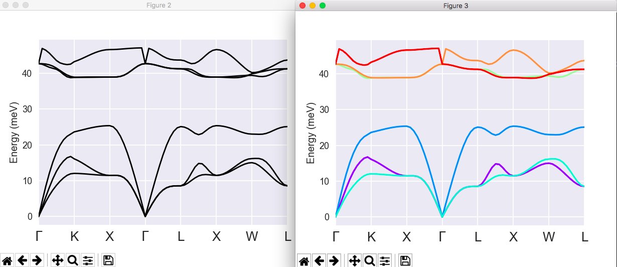
- (left) Phonon bands without LO-TO splitting (right) Plot with band connection estimated from the overlap of the eigenvectors at adjacent q-points
Alternatively, we can start from the DDB file and use the abiview.py script. In this case, AbiPy will generate the anaddb input file with all the variables required to handle the plotting of the LO-TO splitting, invoke anaddb for us and finally plot the results. All of this with just two commands! First, copy the ddb file to a file with extension DDB, then, execute abiview.py:
cp trf2_3.ddb.abo trf2_3_DDB;
abiview.py ddb trf2_3_DDB -sns=talk

We can also compare our results with the phonon band structure available on the materials project .
First of all, let’s find the materials project identifier associated to this particular phase of AlAs. Of course, one could use the materials project web interface but we can also do it from the shell by just passing our Abinit input file to the abistruct.py script:
abistruct.py mp_match trf2_1.abi

# Found 1 structures in Materials Project database (use `verbose` to get further info)

######################### abivars input for mp-2172 #########################
# Full Formula (Al1 As1)
# Reduced Formula: AlAs
# abc   :   4.054377   4.054377   4.054377
# angles:  60.000000  60.000000  60.000000
#
# Spglib space group info (magnetic symmetries are not taken into account).
# Spacegroup: F-43m (216), Hall: F -4 2 3, Abinit spg_number: None
# Crystal_system: cubic, Lattice_type: cubic, Point_group: -43m
#
#   Idx  Symbol    Reduced_Coords              Wyck      EqIdx
# -----  --------  --------------------------  ------  -------
#     0  Al        +0.00000 +0.00000 +0.00000  a             0
#     1  As        +0.25000 +0.25000 +0.25000  d             1

 natom 2
 ntypat 2
 typat 1 2
 znucl 13 33
 xred
    0.0000000000    0.0000000000    0.0000000000
    0.2500000000    0.2500000000    0.2500000000
 acell    1.0    1.0    1.0
 rprim
    6.6351943530    0.0000000000    3.8308312587
    2.2117314510    6.2557212277    3.8308312587
    0.0000000000    0.0000000000    7.6616624984
AbiPy found one entry in the MP database that matches the structure given in our input file
and has generated the corresponding input file.
Now we know that this phase of AlAs corresponds to mp-2172 and we can
look at the phonon band structure computed by [Petretto2018a] at
https://materialsproject.org/materials/mp-2172/
Tip
For further information on the AbiPy API, please consult the DdbFile notebook . To learn how to automate DFPT calculations with Python, see this jupyter notebook.
6 Thermodynamical properties
We will give only a very short example of the use of ANADDB to compute thermodynamical properties. This is because this part of ANADDB is likely the farthest from a clean, stable, usage. By exploring the input variables, the user should be able to produce figures and data like the ones for SiO2 quartz and stishovite, published in [Lee1995].
You can copy the file trf2_6.abi from $ABI_TESTS/tutorespfn/Input to Work_rf2. The same DDB as for trf2_4 and trf2_5 is used, namely trf2_3.ddb.abo.
!Input file for the anaddb code. Analysis of the AlAs ddb

! ddb file
ddb_filepath = "trf2_3.ddb.abo"

! output file
output_file = "trf2_6.abo"
outdata_prefix = "trf2_6o"

!Flags
 ifcflag   1     ! Interatomic force constant flag
 ifcout    0
 thmflag   1     ! Thermodynamical properties flag

!Wavevector grid number 1 (coarse grid, from DDB)
  brav    1         ! Bravais Lattice : 1-S.C., 2-F.C., 3-B.C., 4-Hex.)
  ngqpt   4  4  4   ! Monkhorst-Pack indices
  nqshft  1         ! number of q-points in repeated basic q-cell
  q1shft  3*0.0

!Interatomic force constant info
  dipdip  1      ! Dipole-dipole interaction treatment

!Wavevector grid number 2 (series of fine grids, extrapolated from interat forces)
  ng2qpt   20 20 20  ! sample the BZ up to ngqpt2
  ngrids   5         ! number of grids of increasing size
  q2shft   3*0.0

!Thermal information
  nchan   1250   ! # of channels for the DOS with channel width 1 cm-1
  nwchan  5      ! # of different channel widths from this integer down to 1 cm-1
  thmtol  0.120  ! Tolerance on thermodynamical function fluctuations
  ntemper 10     ! Number of temperatures
  temperinc 20.  ! Increment of temperature in K for temperature dependency
  tempermin 20.  ! Minimal temperature in Kelvin

#%%<BEGIN TEST_INFO>
#%% [setup]
#%% executable = anaddb
#%% test_chain = trf2_1.abi, trf2_2.abi, trf2_3.abi, trf2_4.abi, trf2_5.abi, trf2_6.abi
#%% [files]
#%% files_to_test = trf2_6.abo, tolnlines=  0, tolabs=  0.000e+00, tolrel=  0.000e+00
#%% [paral_info]
#%% max_nprocs = 4
#%% [extra_info]
#%% authors = X. Gonze, J. Zwanziger
#%% keywords =
#%% description = Input file for the anaddb code. Analysis of the SiO2 DDB
#%%<END TEST_INFO>
The following additional input variables are present:
Examine the input file, the input variables, then run anaddb as usual. Then, open the output file. You should be able to find the crucial section:
# At  T     F(J/mol-c)     E(J/mol-c)     S(J/(mol-c.K)) C(J/(mol-c.K)) Omega_mean(cm-1)
# (A mol-c is the abbreviation of a mole-cell, that is, the
#  number of Avogadro times the atoms in a unit cell)
 2.000E+01  8.1406018E+03  8.1484316E+03  3.9149240E-01  1.4057917E+00  7.2615609E+01
 4.000E+01  8.1084535E+03  8.2384509E+03  3.2499352E+00  7.8730812E+00  9.4376064E+01
 6.000E+01  8.0007856E+03  8.4587550E+03  7.6328229E+00  1.3972961E+01  1.1313071E+02
 8.000E+01  7.8007781E+03  8.7924243E+03  1.2395577E+01  1.9312368E+01  1.3603493E+02
 1.000E+02  7.5044659E+03  9.2281056E+03  1.7236397E+01  2.4166544E+01  1.5713727E+02
 1.200E+02  7.1116611E+03  9.7549590E+03  2.2027483E+01  2.8405448E+01  1.7346361E+02
 1.400E+02  6.6242892E+03  1.0359674E+04  2.6681323E+01  3.1951237E+01  1.8536427E+02
 1.600E+02  6.0456925E+03  1.1028647E+04  3.1143464E+01  3.4844495E+01  1.9397760E+02
 1.800E+02  5.3800094E+03  1.1749746E+04  3.5387425E+01  3.7181668E+01  2.0029176E+02
 2.000E+02  4.6317003E+03  1.2512909E+04  3.9406045E+01  3.9067753E+01  2.0500949E+02
There, one finds, the phonon free energy, the phonon internal energy, the phonon entropy and the phonon heat capacity. The atomic temperature factors can also be computed. An example is presented in v5[22]
Important
Do not forget that we are working in the harmonic approximation; beyond some temperature, anharmonic effects will have a sizable contributions.