First tutorial on the Projector Augmented-Wave (PAW) method
Projector Augmented-Wave approach, how to use it?
This tutorial aims at showing how to perform a calculation within the Projector Augmented-Wave (PAW) method.
You will learn how to launch a PAW calculation and what are the main input variables that govern convergence and numerical efficiency. You are supposed to know how to use ABINIT with Norm-Conserving PseudoPotentials (NCPP).
This tutorial should take about 1.5 hour.
Note
Supposing you made your own installation of ABINIT, the input files to run the examples are in the ~abinit/tests/ directory where ~abinit is the absolute path of the abinit top-level directory. If you have NOT made your own install, ask your system administrator where to find the package, especially the executable and test files.
In case you work on your own PC or workstation, to make things easier, we suggest you define some handy environment variables by executing the following lines in the terminal:
export ABI_HOME=Replace_with_absolute_path_to_abinit_top_level_dir # Change this line
export PATH=$ABI_HOME/src/98_main/:$PATH      # Do not change this line: path to executable
export ABI_TESTS=$ABI_HOME/tests/             # Do not change this line: path to tests dir
export ABI_PSPDIR=$ABI_TESTS/Pspdir/  # Do not change this line: path to pseudos dir
Examples in this tutorial use these shell variables: copy and paste
the code snippets into the terminal (remember to set ABI_HOME first!) or, alternatively,
source the set_abienv.sh script located in the ~abinit directory:
source ~abinit/set_abienv.sh
The ‘export PATH’ line adds the directory containing the executables to your PATH so that you can invoke the code by simply typing abinit in the terminal instead of providing the absolute path.
To execute the tutorials, create a working directory (Work*) and
copy there the input files of the lesson.
Most of the tutorials do not rely on parallelism (except specific tutorials on parallelism). However you can run most of the tutorial examples in parallel with MPI, see the topic on parallelism.
1. Summary of the PAW method
The Projector Augmented-Wave approach has been introduced by Peter Blochl in 1994:
The Projector Augmented-Wave method is an extension of augmented wave methods and the pseudopotential approach, which combines their traditions into a unified electronic structure method”. It is based on a linear and invertible transformation (the PAW transformation) that connects the “true” wavefunctions \(\Psi\) with “auxiliary” (or “pseudo”) soft wavefunctions \(\tPsi\):
This relation is based on the definition of augmentation regions (atomic spheres of radius \(r_c\)), around the atoms in which the partial waves \(|\phi_i\rangle\) form a basis of atomic wavefunctions; \(|\tphi_i\rangle\) are pseudized partial waves (obtained from \(|\phi_i\rangle\)), and \(|\tprj_i\rangle\) are dual functions of the \(|\tphi_i\rangle\) called projectors. It is therefore possible to write every quantity depending on \(\Psi_n\) (density, energy, Hamiltonian) as a function of \(\tPsi_n\) and to find \(\tPsi_n\) by solving self-consistent equations.
The PAW method has two main advantages:
- From \(\tPsi\), it is always possible to obtain the true all electron wavefunction \(\Psi\),
- The convergence is comparable to an UltraSoft PseudoPotential (USPP) one.
From a practical point of view, a PAW calculation is rather similar to a Norm-Conserving PseudoPotential one. Most noticeably, one will have to use a special atomic data file (PAW dataset) that contains the \(\phi_i\), \(\tphi_i\) and \(\tprj_i\) and that plays the same role as a pseudopotential file.
Tip
It is highly recommended to read the following papers to understand correctly the basic concepts of the PAW method: [Bloechl1994] and [Kresse1999]. The implementation of the PAW method in ABINIT is detailed in [Torrent2008], describing specific notations and formulations
2. Using PAW with ABINIT
Before continuing, you might consider to work in a different subdirectory as
for the other tutorials. Why not Work_paw1?
In what follows, the name of files are mentioned as if you were in this subdirectory.
All the input files can be found in the $ABI_TESTS/tutorial/Input directory.
Important
You can compare your results with reference output files located in
$ABI_TESTS/tutorial/Refs and $ABI_TESTS/tutorial/Refs/tpaw1_addons
directories (for the present tutorial they are named tpaw1_*.abo).
The input file tpaw1_1.abi is an example of a file to be used to compute the total energy of diamond at the experimental volume (within the LDA exchange-correlation functional). Copy the tpaw1_1.abi file in your work directory,
cd $ABI_TESTS/tutorial/Input
mkdir Work_paw1
cd Work_paw1
cp ../tpaw1_1.abi .
and execute ABINIT:
abinit tpaw1_1.abi >& log
The code should run very quickly. In the meantime, you can read the input file and see that there is no PAW input variable.
# Input for PAW1 tutorial
# Diamond at experimental volume

#Definition of the unit cell
acell 3*3.567 angstrom  # Lengths of the primitive vectors (exp. param. in angstrom)
rprim             # 3 orthogonal primitive vectors (FCC lattice)
  0.0 1/2 1/2
  1/2 0.0 1/2
  1/2 1/2 0.0
nsym 0            # Automatic detection of symetries

#Definition of the atom types and pseudopotentials
ntypat 1          # There is only one type of atom
znucl 6           # Atomic number of the possible type(s) of atom. Here carbon.
pp_dirpath "$ABI_PSPDIR"              # Path to the directory were
                                      #   pseudopotentials for tests are stored
pseudos "PseudosTM_pwteter/6c.pspnc"  # Name and location of the pseudopotential
#pseudos "Psdj_paw_pw_std/C.xml" # To be uncommented later

#Definition of the atoms
natom 2           # There are two atoms
typat 1 1         # They both are of type 1, that is, Carbon
xred              # Location of the atoms:
  0.0 0.0 0.0     #  Triplet giving the reduced coordinates of atom 1
  1/4 1/4 1/4     #  Triplet giving the reduced coordinates of atom 2

#Definition of bands and occupation numbers
nband 6           # Compute 6 bands (4 occupied, 2 empty)
occopt 1          # Automatic generation of occupation numbers, as a semiconductor

#Numerical parameters of the calculation : planewave basis set and k point grid
ecut 15.0         # Maximal plane-wave kinetic energy cut-off, in Hartree
ecutsm 0.5        # Introduce a smooth PW cutoff within an 0.5 Ha region
kptopt 1          # Automatic generation of k points, taking into account the symmetry
ngkpt 6 6 6       # This is a 6x6x6 grid based on the primitive vectors
nshiftk 4         # of the reciprocal space, repeated four times,
shiftk            # with different shifts:
  0.5 0.5 0.5
  0.5 0.0 0.0
  0.0 0.5 0.0
  0.0 0.0 0.5

#Parameters for the SCF procedure
nstep 20          # Maximal number of SCF cycles
tolvrs 1.0d-10    # Will stop when, twice in a row, the difference
                  # between two consecutive evaluations of potential residual
                  # differ by less than tolvrs

#Miscelaneous parameters
prtwf 0           # Do not print wavefunctions
prtden 0          # Do not print density
prteig 0          # Do not print eigenvalues


##############################################################
# This section is used only for regression testing of ABINIT #
##############################################################
#%%<BEGIN TEST_INFO>
#%% [setup]
#%% executable = abinit
#%% [files]
#%% files_to_test =
#%%   tpaw1_1.abo, tolnlines=  0, tolabs=  0.000e+00, tolrel=  0.000e+00
#%% output_file = "tpaw1_1.abo"
#%% [paral_info]
#%% max_nprocs = 4
#%% [extra_info]
#%% authors = M. Torrent
#%% keywords = PAW
#%% description =
#%%   Input for PAW1 tutorial
#%%   Diamond at experimental volume
#%%<END TEST_INFO>
Now, open the tpaw1_1.abi file and change the line with pseudopotential information: replace the PseudosTM_pwteter/6c.pspnc file with Pseudodojo_paw_pw_standard/C.xml. Run the code again:
abinit tpaw1_1.abi >& log
Your run should stop almost immediately! The input file, indeed, is missing the mandatory argument pawecutdg !
Add the line:
pawecutdg 50
to tpaw1_1.abi and run it again. Now the code completes successfully.
Note
The time needed for the PAW run is greater than the time needed for the Norm-Conserving PseudoPotential run; indeed, at constant value of plane wave cut-off energy ecut PAW requires more computational resources:
- the on-site contributions have to be computed,
- the nonlocal contribution of the PAW dataset uses 2 projectors per angular momentum, while the nonlocal contribution of the present Norm-Conserving Pseudopotential uses only one.
However, for many nuclei in the periodic table the plane wave cut-off energy required by PAW is smaller than the cut-off needed for the Norm-Conserving PseudoPotential (see next section), a PAW calculation might actually require less CPU time.
Let’s open the output file (tpaw1_1.abo) and have a look inside (remember: you can compare with a reference file in $ABI_TESTS/tutorial/Refs/). Compared to an output file for a Norm-Conserving PseudoPotential run, an output file for PAW contains the following specific topics:
- At the beginning of the file, some specific default PAW input variables (ngfftdg, pawecutdg, and useylm), mentioned in the section:
-outvars: echo values of preprocessed input variables --------
- The use of two FFT grids, mentioned in:
Coarse grid specifications (used for wave-functions):

getcut: wavevector=  0.0000  0.0000  0.0000  ngfft=  18  18  18
        ecut(hartree)=     15.000   => boxcut(ratio)=   2.17276

Fine grid specifications (used for densities):

getcut: wavevector=  0.0000  0.0000  0.0000  ngfft=  32  32  32
        ecut(hartree)=     50.000   => boxcut(ratio)=   2.10918
- A specific description of the PAW dataset (you might follow the tutorial PAW2, devoted to the building of the PAW atomic data, for a complete understanding of the file):
--- Pseudopotential description ------------------------------------------------
- pspini: atom type   1  psp file is /Users/torrentm/WORK/ABINIT/GIT/beauty/tests//Pspdir/Pseudodojo_paw_pw_standard/C.xml
- pspatm: opening atomic psp file    /Users/torrentm/WORK/ABINIT/GIT/beauty/tests//Pspdir/Pseudodojo_paw_pw_standard/C.xml
- pspatm : Reading pseudopotential header in XML form from /Users/torrentm/WORK/ABINIT/GIT/beauty/tests//Pspdir/Pseudodojo_paw_pw_standard/C.xml
 Pseudopotential format is: paw10
 basis_size (lnmax)=  4 (lmn_size=  8), orbitals=   0   0   1   1
 Spheres core radius: rc_sph= 1.50736703
 1 radial meshes are used:
  - mesh 1: r(i)=AA*[exp(BB*(i-1))-1], size=2001 , AA= 0.94549E-03 BB= 0.56729E-02
 Shapefunction is SIN type: shapef(r)=[sin(pi*r/rshp)/(pi*r/rshp)]**2
 Radius for shape functions =  1.30052589
 mmax= 2001
 Radial grid used for partial waves is grid 1
 Radial grid used for projectors is grid 1
 Radial grid used for (t)core density is grid 1
 Radial grid used for Vloc is grid 1
 Radial grid used for pseudo valence density is grid 1
 Mesh size for Vloc has been set to 1756 to avoid numerical noise.
 Compensation charge density is not taken into account in XC energy/potential
 pspatm: atomic psp has been read  and splines computed
- After the SCF cycle section: The value of the integrated compensation charge evaluated by two different numerical methodologies: 1. computed in the augmentation regions on the “spherical” grid, 2. computed in the whole simulation cell on the “FFT” grid… A discussion on these two values will be done in a forthcoming section.
PAW TEST:
==== Compensation charge inside spheres ============
The following values must be close to each other ...
 Compensation charge over spherical meshes =      0.263866295499286
 Compensation charge over fine fft grid    =      0.263862122639226
- Information related the non-local term (pseudopotential intensity \(D_{ij}\)) and the spherical density matrix (augmentation wave occupancies \(\rho_{ij}\)):
==== Results concerning PAW augmentation regions ====

Total pseudopotential strength Dij (hartree):
Atom #  1
  ...
Atom #  2
  ...

Augmentation waves occupancies Rhoij:
Atom #  1
 ...
Atom #  2
 ...
- At the end of the file we find the decomposition of the total energy both by direct calculation and double counting calculation:
--- !EnergyTerms
iteration_state     : {dtset: 1, }
comment             : Components of total free energy in Hartree
kinetic             :  6.90447470595323E+00
hartree             :  9.62706609299964E-01
xc                  : -4.29580260772849E+00
Ewald energy        : -1.27864121210521E+01
psp_core            :  9.19814512188249E-01
local_psp           : -4.66849481780168E+00
spherical_terms     :  1.43754510318459E+00
total_energy        : -1.15261686159562E+01
total_energy_eV     : -3.13642998643870E+02
...

--- !EnergyTermsDC
iteration_state     : {dtset: 1, }
comment             : '"Double-counting" decomposition of free energy'
band_energy         :  3.08710945092562E-01
Ewald energy        : -1.27864121210521E+01
psp_core            :  9.19814512188249E-01
xc_dc               : -7.38241276339915E-01
spherical_terms     :  7.69958781192718E-01
total_energy_dc     : -1.15261691589185E+01
total_energy_dc_eV  : -3.13643013418624E+02
...
Note
The PAW total energy is not the equal to the one obtained in the Norm-Conserving PseudoPotential case. This is due to the arbitrary modification of the energy reference during the pseudopotential construction. In PAW, comparing total energies computed with different atomic datasets is more meaningful: most of the parts of the energy are calculated exactly, and in general you should be able to compare numbers for (valence) energies between different PAW potentials or different codes.
3. Convergence with respect to the plane-wave basis cut-off
As in the usual Norm-Conserving PseudoPotential case, the critical convergence parameter is the cut-off energy defining the size of the plane-wave basis.
3.a. Norm-Conserving PseudoPotential case
The input file tpaw1_2.abi contains data to be used to compute the convergence in ecut for diamond (at experimental volume). There are 9 datasets, with increasing ecut values from 8 Ha to 24 Ha. You might use the tpaw1_2.abi file (with a standard Norm-Conserving PseudoPotential), and run:
abinit tpaw1_1.abi >& log
You should obtain the following total energy values (see tpaw1_2.abo):
etotal1    -1.1628880677E+01
etotal2    -1.1828052470E+01
etotal3    -1.1921833945E+01
etotal4    -1.1976374633E+01
etotal5    -1.2017601960E+01
etotal6    -1.2046855404E+01
etotal7    -1.2062173253E+01
etotal8    -1.2069642342E+01
etotal9    -1.2073328672E+01
Although it is already quite obvious from these data, by further increasing the value of ecut and obtaining a better estimation of the asymptotic limit, you can check that the etotal convergence (at the 1 mHartree level, that is 0.5 mHartree per atom) is not achieved for \(e_{cut} = 14\) Hartree.
3.b. Projector Augmented-Wave case
Use the same input file as in section 3.a. Again, modify the last line of tpaw1_2.abi, replacing the PseudosTM_pwteter/6c.pspnc file by Pseudodojo_paw_pw_standard/C.xml. Run the code again and open the ABINIT output file (.abo). You should obtain the values:
etotal1    -1.1404460615E+01
etotal2    -1.1496598029E+01
etotal3    -1.1518754947E+01
etotal4    -1.1524981521E+01
etotal5    -1.1526736707E+01
etotal6    -1.1527011746E+01
etotal7    -1.1527027274E+01
etotal8    -1.1527104066E+01
etotal9    -1.1527236307E+01
You can check that:
The etotal convergence (at 1 mHartree) is achieved for \(14 \le e_{cut} \le 16\) Hartree (etotal5 is within 1 mHartree of the final value, the estimated asymptotic value being about -11.527Ha);
With the same input parameters, for diamond, this PAW calculation needs a lower cutoff for converged total energy, compared to a similar calculation with a NCPP.
4. Convergence with respect to the double grid FFT cut-off
In a NCPP calculation, the plane wave density grid should be (at least) twice bigger than the wavefunctions grid, in each direction. In a PAW calculation, the plane wave density grid is tunable thanks to the input variable pawecutdg (PAW: ECUT for Double Grid). This is mainly needed to allow the mapping of densities and potentials, located in the augmentation regions (spheres), onto the global FFT grid. The number of points of the Fourier grid located in the spheres must be large enough to preserve a minimal precision. It is determined from the cut-off energy pawecutdg. One of the most sensitive objects affected by this “grid transfer” is the compensation charge density; its integral over the augmentation regions (on spherical grids) must cancel with its integral over the whole simulation cell (on the FFT grid).
Use now the input file tpaw1_3.abi. The only difference with the tpaw1_2.abi file is that ecut is fixed to 12 Ha, while pawecutdg runs from 12 to 39 Ha.
# Input for PAW1 tutorial
# Diamond at experimental volume
# Convergence with respect to the Double Grid plane-wave cut-off

#Define the different datasets
ndtset 10         # 10 datasets
pawecutdg: 12.    # The starting values of the Double Grid plane-wave cut-off energy
pawecutdg+ 3.     # The increment of pawecutdg from one dataset to the other
getwfk -1         # The starting wave-functions are those of the previous dataset

#-------------------------------------------------------------------------------
#The rest of this file is similar to the tpaw1_1.abi file
#  except the ecut value (12 Ha) deduced from the convergence study

#Definition of the unit cell
acell 3*3.567 angstrom  # Lengths of the primitive vectors (exp. param. in angstrom)
rprim             # 3 orthogonal primitive vectors (FCC lattice)
  0.0 1/2 1/2
  1/2 0.0 1/2
  1/2 1/2 0.0
nsym 0            # Automatic detection of symetries

#Definition of the atom types and pseudopotentials
ntypat 1          # There is only one type of atom
znucl 6           # Atomic number of the possible type(s) of atom. Here carbon.
pp_dirpath "$ABI_PSPDIR"                    # Path to the directory were
                                            #   pseudopotentials for tests are stored
pseudos "Psdj_paw_pw_std/C.xml"  # Name and location of the pseudopotential

#Definition of the atoms
natom 2           # There are two atoms
typat 1 1         # They both are of type 1, that is, Carbon
xred              # Location of the atoms:
  0.0 0.0 0.0     #  Triplet giving the reduced coordinates of atom 1
  1/4 1/4 1/4     #  Triplet giving the reduced coordinates of atom 2

#Definition of bands and occupation numbers
nband 6           # Compute 6 bands (4 occupied, 2 empty)
occopt 1          # Automatic generation of occupation numbers, as a semiconductor

#Numerical parameters of the calculation : planewave basis set and k point grid
ecut 12.0         # Maximal plane-wave kinetic energy cut-off, in Hartree
ecutsm 0.5        # Introduce a smooth PW cutoff within an 0.5 Ha region (not used here)
pawecutdg 50.     # Max. plane-wave kinetic energy cut-off, in Ha, for the PAW double grid
kptopt 1          # Automatic generation of k points, taking into account the symmetry
ngkpt 6 6 6       # This is a 6x6x6 grid based on the primitive vectors
nshiftk 4         # of the reciprocal space, repeated four times,
shiftk            # with different shifts:
  0.5 0.5 0.5
  0.5 0.0 0.0
  0.0 0.5 0.0
  0.0 0.0 0.5

#Parameters for the SCF procedure
nstep 20          # Maximal number of SCF cycles
tolvrs 1.0d-10    # Will stop when, twice in a row, the difference
                  # between two consecutive evaluations of potential residual
                  # differ by less than tolvrs

#Miscelaneous parameters
prtwf 1           # Print wavefunctions (re-used from one dataset to the other)
prtden 0          # Do not print density
prteig 0          # Do not print eigenvalues


##############################################################
# This section is used only for regression testing of ABINIT #
##############################################################
#%%<BEGIN TEST_INFO>
#%% [setup]
#%% executable = abinit
#%% [files]
#%% files_to_test =
#%%   tpaw1_3.abo, tolnlines=  0, tolabs=  0.000e+00, tolrel=  0.000e+00, fld_options=-easy
#%% output_file = "tpaw1_3.abo"
#%% [paral_info]
#%% max_nprocs = 4
#%% [extra_info]
#%% authors = M. Torrent
#%% keywords = PAW
#%% description =
#%%   Input for PAW1 tutorial
#%%   Diamond at experimental volume
#%%   Convergence with respect to the Double Grid plane-wave cut-off
#%%<END TEST_INFO>
Launch ABINIT with these files; you should obtain the values (file tpaw1_3.abo):
etotal1    -1.1518201683E+01
etotal2    -1.1518333032E+01
etotal3    -1.1518666700E+01
etotal4    -1.1518802859E+01
etotal5    -1.1518785111E+01
etotal6    -1.1518739739E+01
etotal7    -1.1518716669E+01
etotal8    -1.1518723268E+01
etotal9    -1.1518738376E+01
etotal10   -1.1518752752E+01
We see that the variation of the energy with respect to the pawecutdg parameter is well below the 1 mHa level. In principle, it should be sufficient to choose pawecutdg = 12 Ha in order to obtain an energy change lower than 1 mHa. In practice, it is better to keep a security margin. Here, for pawecutdg = 24 Ha (5th dataset), the energy change is lower than 0.001 mHa: this choice will be more than enough.
Note
Note the steps in the total energy values. They are due to sudden changes in the grid size (see the output values for ngfftdg) which do not occur for each increase of pawecutdg. To avoid troubles due to these steps, it is better to choose a value of pawecutdg slightly higher than the one stricly needed for the target tolerance criterion.
The convergence of the compensation charge has a similar behaviour; it is possible to check it in the output file, just after the SCF cycle by looking at:
PAW TEST:
==== Compensation charge inside spheres ============
 The following values must be close to each other ...
 Compensation charge over spherical meshes =      0.252499599273249
 Compensation charge over fine fft grid    =      0.252497392737764
The two values of the integrated compensation charge density must be close to each other. Note that, for numerical reasons, they cannot be exactly the same (integration over a radial grid does not use the same scheme as integration over a FFT grid).
Given these basic insights in the effects of pawecutdg, HOW TO PROCEED IN PRACTICE ? In particular, how to combine the convergence study with respect to ecut and the one with respect to pawecutdg ?
Strictly speaking, when testing the convergence of some property with respect to ecut, pawecutdg has to remain constant to obtain consistent results. However, there is the constraint that pawecutdg must be higher or equal to ecut. Also, it must be realized that increasing pawecutdg slightly changes the CPU execution time, but above all it is memory-consumiing so one is interested to keep it small. Note that, if ecut is already high, there might be no need for a higher pawecutdg.
Different people have different tricks, of course. The following recipe might do the work. First consider the case where ecut and pawecutdg are equal to each others, and perform a convergence study on the target property (e.g. the total energy) keeping this constraint. You will be determine that some energy value, for which ecut=pawecutdg, meet your tolerance. Below this energy, the convergence criterion is not met. But will this lack of convergence come because of the detrimental effect of ecut or the one of pawecutdg ? If it is due to ecut, in any case you cannot set pawecutdg to a lower value than ecut… Thus, one has to test the other hypothesis. So, fix pawecutdg to that satisfying value, possibly increased by some small security margin, and REDO a convergence study only for ecut, starting with a much lower value.
So, for example, let us modify tpaw1_2.abi file, increasing both ecut and pawecutdg concurrently from 8Ha to 24 Ha by step of 2Ha. The following values are obtained:
       etotal1    -1.1408113469E+01
       etotal2    -1.1497119746E+01
       etotal3    -1.1518201683E+01
       etotal4    -1.1524416771E+01
       etotal5    -1.1526469512E+01
       etotal6    -1.1526927373E+01
       etotal7    -1.1527067048E+01
       etotal8    -1.1527173207E+01
       etotal9    -1.1527266773E+01
One can check again that the etotal convergence (at the 1 mHartree level) is achieved for \(14 \le e_{cut} \le 16\) Ha, with similar value for pawecutdg. But is this convergence limited by ecut or pawecutdg ? The second step is thus to fix pawecutdg to a slightly higher value than 16 Ha, let us say 18 Ha, and explore the effect of ecut only. The highest value of ecut to be tested is 18 Ha, of course (and we already have the value for ecut=pawecutdg=18 Ha). The following values are obtained (for ecut going from 8 Ha to 18 Ha by steps of 2 Ha, and for pawecutdg fixed to 18 Ha):
       etotal1    -1.1404374728E+01
       etotal2    -1.1496509531E+01
       etotal3    -1.1518666700E+01
       etotal4    -1.1524894829E+01
       etotal5    -1.1526651588E+01
       etotal6    -1.1526927373E+01
This indicates that ecut 14 or lower is not sufficient to reach the tolerance criterion. One should stick to ecut 16 and pawecutdg 18 (or may be 16 if memory problems might be present).
5. Plotting PAW contributions to the Density of States (DOS)
We now use the input file tpaw1_4.abi file. ABINIT is used to compute the Density Of State (DOS) (see the prtdos keyword in the input file). Also note that more k-points are used in order to increase the precision of the DOS. ecut is set to 12 Ha, while pawecutdg is 24 Ha.
# Input for PAW1 tutorial
# Diamond at experimental volume
# Computation of Density of States (DOS)

#Specific input parameters related to DOS printing

#Case 1: Total DOS
prtdos 1          # Flag to activate the total DOS output

#Case 2: projected DOS  (to be uncommented later)
#prtdos 3          # Flag to activate the projected DOS output
#pawprtdos 1       # Flag to activate the output of all PAW contributions
#natsph 1          # Number of atom(s) around which the projected DOS has to computed
#iatsph 1          #  Index of these atoms
#ratsph 1.51       #  Radius defining the projection area around the atom(s)

#For this calculation we take a metallic scheme for the occupation numbers
#This is mandatory for a DOS calculation
occopt 7           # Automatic generation of occupation numbers, as a metal
tsmear 0.005       # Smearing temperature for the metallic occupation scheme (Hartree)

#For this calculation we take more k-points to have a smoother DOS curve
ngkpt 10 10 10     # This is a 10x10x10 grid based on the primitive vectors

#-------------------------------------------------------------------------------
#The rest of this file is similar to the tpaw1_1.abi file
#  using the ecut and pawecutdg values deduced from the convergence studies

#Definition of the unit cell
acell 3*3.567 angstrom  # Lengths of the primitive vectors (exp. param. in angstrom)
rprim             # 3 orthogonal primitive vectors (FCC lattice)
  0.0 1/2 1/2
  1/2 0.0 1/2
  1/2 1/2 0.0
nsym 0            # Automatic detection of symetries

#Definition of the atom types and pseudopotentials
ntypat 1          # There is only one type of atom
znucl 6           # Atomic number of the possible type(s) of atom. Here carbon.
pp_dirpath "$ABI_PSPDIR"                    # Path to the directory were
                                            #   pseudopotentials for tests are stored
pseudos "Psdj_paw_pw_std/C.xml"  # Name and location of the pseudopotential
#pseudos "C_paw_pw_2proj.xml"               # Uncomment this line later
#pseudos "C_paw_pw_2proj.xml"               # Uncomment this line later


#Definition of the atoms
natom 2           # There are two atoms
typat 1 1         # They both are of type 1, that is, Carbon
xred              # Location of the atoms:
  0.0 0.0 0.0     #  Triplet giving the reduced coordinates of atom 1
  1/4 1/4 1/4     #  Triplet giving the reduced coordinates of atom 2

#Definition of bands and occupation numbers
nband 6           # Compute 6 bands (4 occupied, 2 empty)

#Numerical parameters of the calculation : planewave basis set and k point grid
ecut 12.0         # Maximal plane-wave kinetic energy cut-off, in Hartree
ecutsm 0.5        # Introduce a smooth PW cutoff within an 0.5 Ha region (not used here)
pawecutdg 24.     # Max. plane-wave kinetic energy cut-off, in Ha, for the PAW double grid
kptopt 1          # Automatic generation of k points, taking into account the symmetry
nshiftk 4         # of the reciprocal space, repeated four times,
shiftk            # with different shifts:
  0.5 0.5 0.5
  0.5 0.0 0.0
  0.0 0.5 0.0
  0.0 0.0 0.5

#Parameters for the SCF procedure
nstep 20          # Maximal number of SCF cycles
tolvrs 1.0d-10    # Will stop when, twice in a row, the difference
                  # between two consecutive evaluations of potential residual
                  # differ by less than tolvrs

#Miscelaneous parameters
prtwf  0          # Do not print wavefunctions
prtden 0          # Do not print density
prteig 0          # Do not print eigenvalues


##############################################################
# This section is used only for regression testing of ABINIT #
##############################################################
#%%<BEGIN TEST_INFO>
#%% [setup]
#%% executable = abinit
#%% [files]
#%% files_to_test =
#%%   tpaw1_4.abo, tolnlines=  0, tolabs=  0.000e+00, tolrel=  0.000e+00, fld_options = -easy
#%% output_file = "tpaw1_4.abo"
#%% [paral_info]
#%% max_nprocs = 4
#%% [extra_info]
#%% authors = M. Torrent
#%% keywords = PAW
#%% description =
#%%   Input for PAW1 tutorial
#%%   Diamond at experimental volume
#%%   Computation of Density of States
#%%<END TEST_INFO>
Launch the code with these files; you should obtain the tpaw1_4.abo and the DOS file (tpaw1_4o_DOS):
abinit tpaw1_4.abi >& log
You can plot the DOS file; for this purpose, use a graphical tool and plot column 3 with respect to column 2. Example: if you use the xmgrace tool, launch:
xmgrace -block tpaw1_4o_DOS -bxy 1:2
At this stage, you have a usual Density of State plot; nothing specific to PAW.
Now, edit the tpaw1_4.abi file, comment the “prtdos 1” line, and uncomment (or add):
prtdos 3
pawprtdos 1
natsph 1 iatsph 1
ratsph 1.51
prtdos=3 requires the output of the projected DOS; natsph=1, iatsph=1 select the first carbon atom as the center of projection, and ratsph=1.51 sets the radius of the projection area to 1.51 atomic units (this is exactly the radius of the PAW augmentation regions: generally the best choice). pawprtdos=1 is specific to PAW. With this option, ABINIT should compute all the contributions to the projected DOS.
Let us remember that:
Within PAW, the total projected DOS has 3 contributions:
- The smooth plane-waves (PW) contribution (from \(|\tPsi\rangle\)),
- The all-electron on-site (AE) contribution (from \(\langle \tprj^a_i|\tPsi\rangle |\phi_i^a\rangle\)),
- The pseudo on-site (PS) contribution (from \(\langle \tprj^a_i|\tPsi\rangle |\tphi_i^a\rangle\)).
Execute ABINIT again (with the modified input file). You get a new DOS file, named tpaw1_4o_DOS_AT0001. You can edit it and look inside; it contains the 3 PAW contributions (mentioned above) for each angular momentum. In the diamond case, only \(l = 0\) and \(l = 1\) momenta are to be considered.
Now, plot the file, using the 7th, 12th and 17th columns with respect to the 2nd one; it plots the 3 PAW contributions for \(l = 0\) (the total DOS is the sum of the three contributions). If you use the xmgrace tool, launch:
xmgrace -block tpaw1_4o_DOS_AT0001 -bxy 1:7 -bxy 1:12 -bxy 1:17
You should get this:
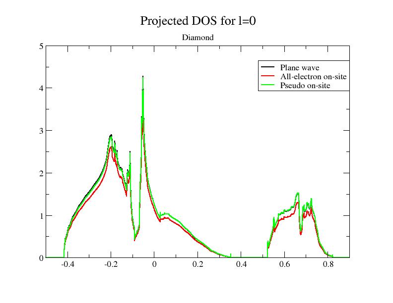
As you can see, the smooth PW contribution and the PS on-site contribution are close. At basis completeness, they should cancel; we could approximate the DOS by the AE on-site part taken alone. That’s exactly the purpose of the pawprtdos = 2 option: in that case, only the AE on-site contribution is computed and given as a good approximation of the total projected DOS. The main advantage of this option is that the computing time is greatly reduced (the DOS is instantaneously computed).
However, as you will see in the next section, this approximation is only valid when:
- The \(\tphi_i\) basis is complete enough
- The electronic density is mainly contained in the sphere defined by ratsph.
6. Testing the completeness of the PAW partial wave basis
In the previous section we used a “standard” PAW dataset, with 2 partial waves per angular momentum. It is generally the best compromise between the completeness of the partial wave basis and the efficiency of the PAW dataset (the more partial waves you have, the longer the CPU time used by ABINIT is).
Let’s have a look at the $ABI_PSPDIR/Pseudodojo_paw_pw_standard/C.xml file. The tag <valence_states has 4 <state lines. This indicates the number of partial waves (4) and their \(l\) angular momentum. In the present file, there are two \(l = 0\) partial waves and two \(l = 1\) partial waves.
Now, let’s open the $ABI_PSPDIR/C_paw_pw_2proj.xml and $ABI_PSPDIR/C_paw_pw_6proj.xml PAW dataset files. The first dataset is based on only one partial wave per \(l\); the second one is based on three partial waves per \(l\). The completeness of the partial wave basis increases when you use C_paw_pw_2proj.xml, Pseudodojo_paw_pw_standard/C.xml and C_paw_pw_6proj.xml.
Now, let us plot the DOS using the two new PAW datasets.
- Save the existing tpaw1_4o_DOS_AT0001 file, naming it f.i. tpaw1_4o_4proj_DOS_AT0001.
- Open the tpaw1_4.abi file and modify it in order to use the C_paw_pw_2proj.xml PAW dataset.
- Run ABINIT.
- Save the new tpaw1_4o_DOS_AT0001 file, naming it f.i. tpaw1_4o_2proj_DOS_AT0001.
- Open the tpaw1_4.abi file and modify it in order to use the C_paw_pw_2proj.xml PAW dataset.
- Run ABINIT again.
- Save the new tpaw1_4o_DOS_AT0001 file, naming it f.i. tpaw1_4o_6proj_DOS_AT0001.
Then, plot the contributions to the projected DOS for the two new DOS files. You should get:
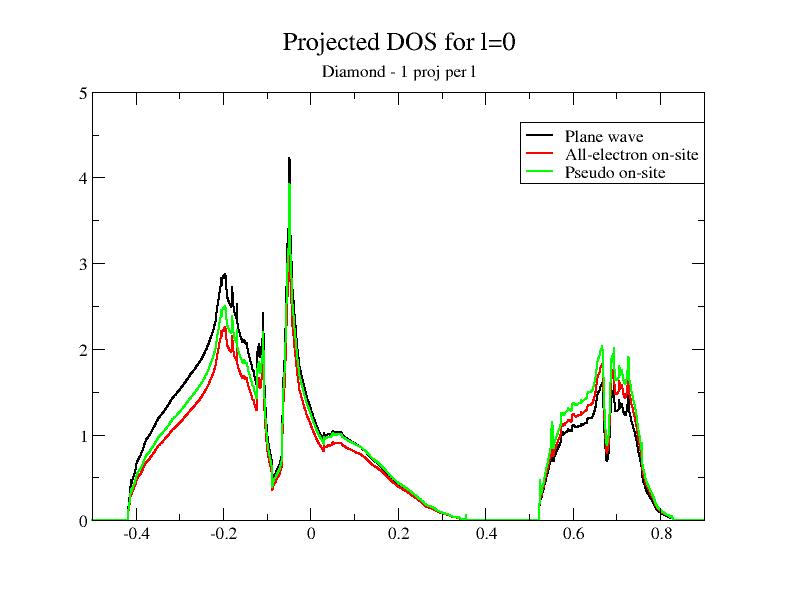
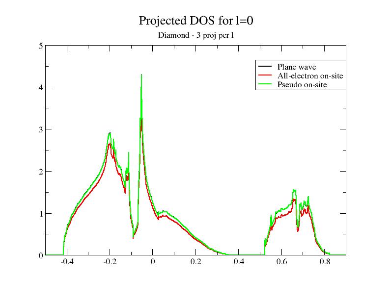
Adding the DOS obtained in the previous section to the comparison, you immediately see that the superposition of the plane wave part DOS (PW) and the PS on-site DOS depends on the completeness of the partial wave basis!
Now, you can have a look at the 3 output files (one for each PAW dataset). A way to estimate the completeness of the partial wave basis is to compare derivatives of total energy; if you look at the stress tensor:
For the 2 `partial-wave` basis:   2.85307799E-04  2.85307799E-04 2.85307799E-04  0.  0.  0.
For the 4 `partial-wave` basis:   4.97872484E-04  4.97872484E-04 4.97872484E-04  0.  0.  0.
For the 6 `partial-wave` basis:   5.38392693E-04  5.38392693E-04 5.38392693E-04  0.  0.  0.
The 2 partial-wave basis is clearly not complete; the 4 partial-wave basis results are correct. Such a test is useful to estimate the precision we can expect on the stress tensor (at least due to the partial wave basis completeness).
You can compare other results in the 3 output files: total energy, eigenvalues, occupations…
Note
The CPU time increases with the size of the partial wave basis. This is why it is not recommended to use systematically high-precision PAW datasets. If you want to learn how to generate PAW datasets with different partial wave basis, you might follow the tutorial on generating PAW datasets (PAW2).
7. Checking the validity of PAW results
The validity of our computation has to be checked by comparison, on known structures, with known results. In the case of diamond, lots of computations and experimental results exist.
Important
The validity of PAW calculations (completeness of plane wave basis and partial wave basis) should always be checked by comparison with all-electrons computations or with other existing PAW results; it should not be done by comparison with experimental results. As the PAW method has the same accuracy than all-electron methods, results should be very close.
In the case of diamond, all-electron results can be found f.i. in [Holzwarth1997]. All-electron equilibrium parameters for diamond (within Local Density Approximation) obtained with the FP-LAPW WIEN2K code are:
a0 = 3.54 angstrom
B = 470 GPa
Experiments give:
a0 = 3.56 angstrom
B = 443 GPa
Let’s test with ABINIT. We use now the input file tpaw1_5.abi file and we run ABINIT to compute values of etotal for several cell parameters around 3.54 angstrom, using the standard PAW dataset.
# Input for PAW1 tutorial
# Diamond: etotal vs acell curve around equilibrium

#Define the different datasets
ndtset 7                 # 7 datasets
acell: 3*3.515 angstrom  # The starting values of the primitive vector lengths
acell+ 3*0.005 angstrom  # The increment of acell from one dataset to the other
getwfk -1                # The starting wave-functions are those of the previous dataset

#-------------------------------------------------------------------------------
#The rest of this file is similar to the tpaw1_4.abi file
#  with ecut=20, pawecutdg=50 and ngkpt=3*10 for higher precision

#Definition of the unit cell
acell 3*3.567 angstrom  # Lengths of the primitive vectors (not used here)
rprim             # 3 orthogonal primitive vectors (FCC lattice)
  0.0 1/2 1/2
  1/2 0.0 1/2
  1/2 1/2 0.0
nsym 0            # Automatic detection of symetries

#Definition of the atom types and pseudopotentials
ntypat 1          # There is only one type of atom
znucl 6           # Atomic number of the possible type(s) of atom. Here carbon.
pp_dirpath "$ABI_PSPDIR"                    # Path to the directory were
                                            #   pseudopotentials for tests are stored
pseudos "Psdj_paw_pw_std/C.xml"  # Name and location of the pseudopotential

#Definition of the atoms
natom 2           # There are two atoms
typat 1 1         # They both are of type 1, that is, Carbon
xred              # Location of the atoms:
  0.0 0.0 0.0     #  Triplet giving the reduced coordinates of atom 1
  1/4 1/4 1/4     #  Triplet giving the reduced coordinates of atom 2

#Definition of bands and occupation numbers
nband 6           # Compute 6 bands (4 occupied, 2 empty)
occopt 1          # Automatic generation of occupation numbers, as a semiconductor

#Numerical parameters of the calculation : planewave basis set and k point grid
ecut 20.0         # Maximal plane-wave kinetic energy cut-off, in Hartree
ecutsm 0.5        # Introduce a smooth PW cutoff within an 0.5 Ha region (not used here)
pawecutdg 50.     # Max. plane-wave kinetic energy cut-off, in Ha, for the PAW double grid
kptopt 1          # Automatic generation of k points, taking into account the symmetry
ngkpt 10 10 10    # This is a 10x10x10 grid based on the primitive vectors
nshiftk 4         # of the reciprocal space, repeated four times,
shiftk            # with different shifts:
  0.5 0.5 0.5
  0.5 0.0 0.0
  0.0 0.5 0.0
  0.0 0.0 0.5

#Parameters for the SCF procedure
nstep 10          # Maximal number of SCF cycles
tolvrs 1.0d-10    # Will stop when, twice in a row, the difference
                  # between two consecutive evaluations of potential residual
                  # differ by less than tolvrs

#Miscelaneous parameters
prtwf 1           # Print wavefunctions (re-used from one dataset to the other)
prtden 0          # Do not print density
prteig 0          # Do not print eigenvalues


##############################################################
# This section is used only for regression testing of ABINIT #
##############################################################
#%%<BEGIN TEST_INFO>
#%% [setup]
#%% executable = abinit
#%% [files]
#%% files_to_test =
#%%   tpaw1_5.abo, tolnlines=  0, tolabs=  0.000e+00, tolrel=  0.000e+00, fld_options = -easy
#%% output_file = "tpaw1_5.abo"
#%% [paral_info]
#%% max_nprocs = 4
#%% [extra_info]
#%% authors = M. Torrent
#%% keywords = PAW
#%% description =
#%%   Input for PAW1 tutorial
#%%   Diamond: etotal vs acell curve around equilibrium
#%%<END TEST_INFO>
abinit tpaw1_1.abi >& log
From the tpaw1_5.abo file, you can extract the 7 values of acell and 7 values of etotal, then put them into a file and plot it with a graphical tool. You should get:
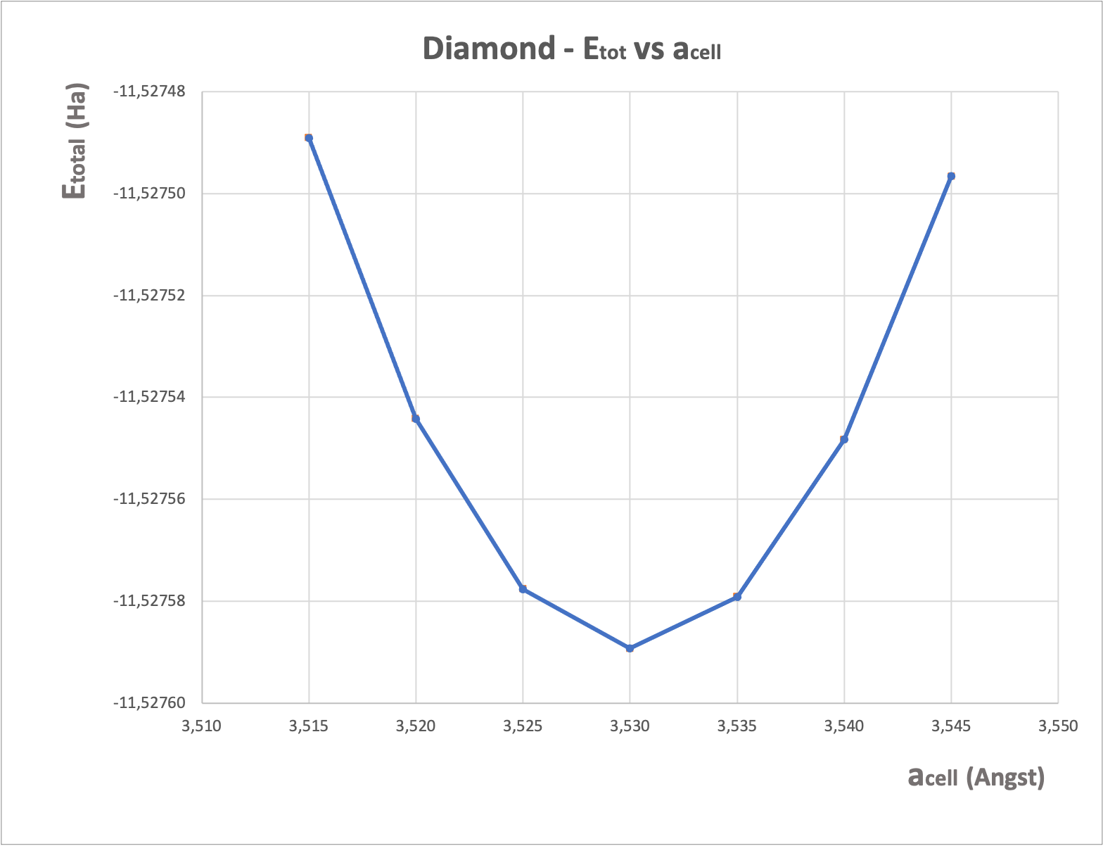
From this curve, you can extract the cell values of \(a_0\) and \(B\) (with the method of your choice, for example by a Birch-Murnhagan spline fit). You get:
a0 = 3.53 angstrom B = 469.5 GPa
These results are in excellent agreement with FP-LAPW ones!
8. Additional comments about PAW in ABINIT
8.a. Overlap of PAW augmentation regions
In principle, the PAW formalism is only valid for non-overlapping augmentation spherical regions. But, in usual cases, a small overlap between spheres is acceptable. By default, ABINIT checks that the distances between atoms are large enough to avoid overlap; a “small” voluminal overlap of 5% is accepted by default. This value can be tuned with the pawovlp input keyword. The overlap check can even be by-passed with pawovlp=-1 (not recommended!).
Warning
While a small overlap can be acceptable for the augmentation regions, an overlap of the compensation charge densities has to be avoided. The compensation charge density is defined by a radius (named \(r_{shape}\) in the PAW dataset) and an analytical shape function. The overlap related to the compensation charge radius is checked by ABINIT and a WARNING is eventually printed.
Also note that you can control the compensation charge radius and shape function while generating the PAW dataset (see tutorial on generating PAW datasets (PAW2)).
8.b. Mixing scheme for the Self-Consistent cycle; decomposition of the total energy
The use of an efficient mixing scheme in the self-consistent loop is a crucial point to minimize the number of steps to achieve convergence. This mixing can be done on the potential or on the density. By default, in a Norm-Conserving PseudoPotential calculation, the mixing is done on the potential; but, for technical reasons, this choice is not optimal for PAW calculations. Thus, by default, the mixing is done on the density when PAW is activated.
The mixing scheme can be controlled by the iscf variable (see the different options of this input variable). To compare both schemes, you can edit the tpaw1_1.abi file and try iscf = 7 or 17 and compare the behaviour of the SC cycle in both cases; as you can see, the final total energy is the same but the way to reach it is completely different.
Now, have a look at the end of the file and focus on the Components of total
free energy; the total energy is decomposed according to two different schemes (direct and double counting);
at very high convergence of the SCF cycle the potential/density
residual is very small and these two values should be the same.
But it has been observed that
the converged value was reached more rapidly by the direct energy, when the
mixing is on the potential, and by the double counting energy when the mixing
is on the density. Thus, by default, in the output file is to print the direct
energy when the mixing is on the potential, and the double counting energy
when the mixing is on the density.
Also note that PAW partial waves occupancies \(\rho_{ij}\) also are mixed during the SC cycle; by default, the mixing is done in the same way as the density.
8.c. PAW+U for correlated materials
If the system under study contains strongly correlated electrons, the DFT+U
method can be useful. It is controlled by the usepawu, lpawu,
upawu and jpawu input keywords.
Note that the formalism implemented in ABINIT is approximate, i.e. it is only valid if:
- The \(\tphi^a_i\) basis is complete enough;
- The electronic density is mainly contained in the PAW sphere.
The approximation done here is the same as the one explained in the 5th section of this tutorial: considering that smooth PW contributions and PS on-site contributions are closely related, only the AE on-site contribution is computed; it is indeed a very good approximation.
Converging a Self-Consistent Cycle, or ensuring the global minimum is reached, with PAW+U is sometimes difficult. Using usedmatpu and dmatpawu can help. See tutorial on DFT+U.
8.d. Printing volume for PAW
If you want to get more detailed output concerning the PAW computation, you can use the pawprtvol input keyword. It is particularly useful to print details about pseudopotential strength \(D_{ij}\) or partial waves occupancies \(\rho_{ij}\).
8.e. Additional PAW input variables
Looking at the PAW variable set, you can find the description of additional input keywords related to PAW. They are to be used when tuning the computation, in order to gain precision or save CPU time.
See also descriptions of these variables and input file examples in the PAW topic page.
Warning
In a standard computation, these variables should not be modified!