Parallelism for many-body calculations
G0W0 corrections in α-quartz SiO2.
This tutorial aims at showing how to perform parallel calculations with the GW part of ABINIT. We will discuss the approaches used to parallelize the different steps of a typical G0W0 calculation, and how to setup the parameters of the run in order to achieve good speedup. α-quartz SiO2 is used as test case.
It is supposed that you have some knowledge about UNIX/Linux, and you know how to submit MPI jobs. You are supposed to know already some basics of parallelism in ABINIT, explained in the tutorial A first introduction to ABINIT in parallel.
In the following, when “run ABINIT over nn CPU cores” appears, you have to use a specific command line according to the operating system and architecture of the computer you are using. This can be for instance:
mpirun -n nn abinit abinit.abi
or the use of a specific submission file.
This tutorial should take about 1.5 hour and requires a modern computer cluster of 20 CPU cores or more.
Note
Supposing you made your own installation of ABINIT, the input files to run the examples are in the ~abinit/tests/ directory where ~abinit is the absolute path of the abinit top-level directory. If you have NOT made your own install, ask your system administrator where to find the package, especially the executable and test files.
In case you work on your own PC or workstation, to make things easier, we suggest you define some handy environment variables by executing the following lines in the terminal:
export ABI_HOME=Replace_with_absolute_path_to_abinit_top_level_dir # Change this line
export PATH=$ABI_HOME/src/98_main/:$PATH      # Do not change this line: path to executable
export ABI_TESTS=$ABI_HOME/tests/             # Do not change this line: path to tests dir
export ABI_PSPDIR=$ABI_TESTS/Pspdir/  # Do not change this line: path to pseudos dir
Examples in this tutorial use these shell variables: copy and paste
the code snippets into the terminal (remember to set ABI_HOME first!) or, alternatively,
source the set_abienv.sh script located in the ~abinit directory:
source ~abinit/set_abienv.sh
The ‘export PATH’ line adds the directory containing the executables to your PATH so that you can invoke the code by simply typing abinit in the terminal instead of providing the absolute path.
To execute the tutorials, create a working directory (Work*) and
copy there the input files of the lesson.
Most of the tutorials do not rely on parallelism (except specific tutorials on parallelism). However you can run most of the tutorial examples in parallel with MPI, see the topic on parallelism.
1 Generating the WFK file in parallel
Before beginning, you should create a working directory in $ABI_TESTS/tutoparal/Input whose name might be Work_mbt.
cd $ABI_TESTS/tutoparal/Input/
mkdir Work_mbt && cd Work_mbt
The input files necessary to run the examples related to this tutorial are located in the directory $ABI_TESTS/tutoparal/Input . We will do most of the actions of this tutorial in this working directory.
Note that the pseudopotentials needed for running the tutorial (Si.psp8 and O.psp8) are located in the directory $ABI_PSPDIR/Pseudodojo_nc_sr_04_pw_standard_psp8.
In the first GW tutorial, we have learned how to generate the WFK file with the sequential version of the code. Now we will perform a similar calculation taking advantage of the k-point parallelism implemented in the ground-state part.
First of all, copy all input files tmbt_*.abi in the working directory Work_mbt:
cd Work_mbt
cp ../tmbt_*.abi .
Now open the input file $ABI_TESTS/tutoparal/Input/tmbt_1.abi in your preferred editor, and look at its structure.
# Crystalline alpha-quartz
ndtset 2
timopt -1

# DATASET 1 : GS calculation
tolvrs1     1d-8
nband1      28     # Adding 4 empty states to avoid problems in the SCF cycle.

# DATASET 2 : WFK generation
iscf2      -2      # NSCF
getden2    -1      # Read previous density
tolwfr2    1d-12   # Stopping criterion for the NSCF cycle.
nband2      160    # Number of (occ and empty) bands computed in the NSCF cycle.
nbdbuf2     10     # A large buffer helps to reduce the number of NSCF steps.

#################### COMMON PART #########################

# number of self-consistent field steps
nstep        200
diemac       4.0

# energy cutoff [Ha]:
ecut         36

#Definition of the k-point grid
occopt 1           # Semiconductor
kptopt 1           # Option for the automatic generation of k points, taking
                   # into account the symmetry

ngkpt   4 4 3
nshiftk  1
shiftk  0.0 0.0 0.0   # The mesh contains the Gamma point
                      # so that we can evaluate the QP correction for this point.
istwfk  *1

# Definition of the atom types
npsp   2
znucl  14  8
ntypat 2

# Definition of the atoms
natom 9
typat 3*1  6*2

# Experimental parameters (Wyckoff pag 312)
# u(Si)= 0.465
# x= 0.415 ; y= 0.272 ; z= 0.120

acell   2*4.91304  5.40463  Angstrom

xred   0.465   0.000   0.000              #Si
       0.000   0.465   2/3                #Si
      -0.465  -0.465   1/3                #Si
       0.415   0.272   0.120              #O
      -0.143  -0.415   0.4533333333333333 #O
      -0.272   0.143   0.7866666666666666 #O
       0.143  -0.272  -0.120              #O
       0.272   0.415   0.5466666666666666 #O
      -0.415  -0.143   0.2133333333333333 #O

rprim   5.0000000000e-01 -8.6602540378e-01  0.0000000000e+00
        5.0000000000e-01  8.6602540378e-01  0.0000000000e+00
        0.0000000000e+00  0.0000000000e+00  1.0000000000e+00

 pp_dirpath "$ABI_PSPDIR"
 pseudos "Psdj_nc_sr_04_pw_std_psp8/Si.psp8, Psdj_nc_sr_04_pw_std_psp8/O.psp8"

##############################################################
# This section is used only for regression testing of ABINIT #
##############################################################
#%%<BEGIN TEST_INFO>
#%% [setup]
#%% executable = abinit
#%% test_chain = tmbt_1.abi, tmbt_2.abi, tmbt_3.abi
##%% test_chain = tmbt_1.abi, tmbt_2.abi, tmbt_3.abi, tmbt_4.abi
#%% [files]
#%% [paral_info]
#%% max_nprocs = 64
#%% nprocs_to_test = 64
#%% [NCPU_64]
#%% files_to_test = tmbt_1_MPI64.abo, tolnlines = 5, tolabs = 1.100e-03, tolrel = 3.000e-03
#%% [shell]
#%% post_commands =
#%%  ww_cp tmbt_1_MPI64o_DS2_WFK tmbt_2_MPI64i_WFK;
#%%  ww_cp tmbt_1_MPI64o_DS2_WFK tmbt_3_MPI64i_WFK;
#%%  ww_cp tmbt_1_MPI64o_DS2_WFK tmbt_4_MPI64i_WFK;
#%% [extra_info]
#%% authors = M. Giantomassi
#%% keywords =  GW
#%% description = GW calculation for crystalline alpha-quartz. Preparatory GS run.
#%%<END TEST_INFO>
The first dataset performs a rather standard SCF calculation to obtain the ground-state density. The second dataset reads the density file and calculates the Kohn-Sham band structure including many empty states:
# DATASET 2 : WFK generation
iscf2      -2      # NSCF
getden2    -1      # Read previous density
tolwfr2    1d-12   # Stopping criterion for the NSCF cycle.
nband2      160    # Number of (occ and empty) bands computed in the NSCF cycle.
nbdbuf2     10     # A large buffer helps to reduce the number of NSCF steps.
We have already encountered these variables in the first GW tutorial so their meaning should be familiar to you. The only thing worth stressing is that this calculation solves the NSCF cycle with the conjugate-gradient method (paral_kgb == 0)
The NSCF cycle is executed in parallel using the standard parallelism over k-points and spin in which the (nkpt x nsppol) blocks of bands are distributed among the nodes. This test uses an unshifted 4x4x3 grid (48 k points in the full Brillouin Zone, folding to 9 k-points in the irreducible wedge) hence the theoretical maximum speedup is 9.
Now run ABINIT over nn CPU cores using (here, nn=9)
mpirun -n 9 abinit tmbt_1.abi > tmbt_1.log 2> err &
but keep in mind that, to avoid idle processors, the number of CPUs (nn) should divide 9. At the end of the run, the code will produce the file tmbt_1o_DS2_WFK needed for the subsequent GW calculations.
With three cores, the wall clock time is around 1.5 minutes.
>>> tail tmbt_1.out

-
- Proc.   0 individual time (sec): cpu=        209.0  wall=        209.0

================================================================================

 Calculation completed.
.Delivered    0 WARNINGs and   5 COMMENTs to log file.
+Overall time at end (sec) : cpu=        626.9  wall=        626.9
A reference output file is given in $ABI_TESTS/tutoparal/Refs, under the name tmbt_1.abo.
Note that 150 bands are not enough to obtain converged GW results, you might increase the number of bands in proportion to your computing resources.
2 Computing the screening in parallel using the Adler-Wiser expression
In this part of the tutorial, we will compute the RPA polarizability with the Adler-Wiser approach. The basic equations are discussed in this section of the GW notes.
First copy the file tmbt_2.abi in the working directory, then create a symbolic link pointing to the WFK file we have generated in the previous step:
>>> ln -s tmbt_1o_DS2_WFK tmbt_2i_WFK
Now open the input file $ABI_TESTS/tutoparal/Input/tmbt_2.abi so that we can discuss its structure.
# Crystalline alpha-quartz
# DATASET 1 : Screening calculation
#
optdriver   3   # Screening run
irdwfk      1   # To read the WFK file
symchi      1   # Use symmetries to speedup the BZ integration
gwpara      2   # Parallelization over bands
awtr        1   # Take advantage of time-reversal. Mandatory when gwpara=2 is used.
ecutwfn     36  # Cutoff for the wavefunctions.
ecuteps     8   # Cutoff for the polarizability.
nband       50  # Number of bands in the RPA expression (24 occupied bands)
inclvkb     2   # Correct treatment of the optical limit.

timopt -1

#################### COMMON PART #########################

# number of self-consistent field steps
nstep        200

# energy cutoff [Ha]:
ecut         36

#Definition of the k-point grid
occopt 1           # Semiconductor
kptopt 1           # Option for the automatic generation of k points, taking
                   # into account the symmetry

ngkpt   4 4 3
nshiftk  1
shiftk  0.0 0.0 0.0
istwfk  *1

# Definition of the atom types
npsp   2
znucl  14  8
ntypat 2

# Definition of the atoms
natom 9
typat 3*1  6*2

# Experimental parameters (Wyckoff pag 312)
# u(Si)= 0.465
# x= 0.415 ; y= 0.272 ; z= 0.120

acell   2*4.91304  5.40463  Angstrom

xred   0.465   0.000   0.000              #Si
       0.000   0.465   2/3                #Si
      -0.465  -0.465   1/3                #Si
       0.415   0.272   0.120              #O
      -0.143  -0.415   0.4533333333333333 #O
      -0.272   0.143   0.7866666666666666 #O
       0.143  -0.272  -0.120              #O
       0.272   0.415   0.5466666666666666 #O
      -0.415  -0.143   0.2133333333333333 #O

rprim   5.0000000000e-01 -8.6602540378e-01  0.0000000000e+00
        5.0000000000e-01  8.6602540378e-01  0.0000000000e+00
        0.0000000000e+00  0.0000000000e+00  1.0000000000e+00

 pp_dirpath "$ABI_PSPDIR"
 pseudos "Psdj_nc_sr_04_pw_std_psp8/Si.psp8, Psdj_nc_sr_04_pw_std_psp8/O.psp8"

##############################################################
# This section is used only for regression testing of ABINIT #
##############################################################
#%%<BEGIN TEST_INFO>
#%% [setup]
#%% executable = abinit
#%% test_chain = tmbt_1.abi, tmbt_2.abi, tmbt_3.abi
##%% test_chain = tmbt_1.abi, tmbt_2.abi, tmbt_3.abi, tmbt_4.abi
#%% [files]
#%% [paral_info]
#%% max_nprocs = 64
#%% nprocs_to_test = 64
#%% [NCPU_64]
#%% files_to_test = tmbt_2_MPI64.abo, tolnlines = 10, tolabs = 1.100e-03, tolrel = 3.000e-03
#%% [shell]
#%% post_commands =
#%%  ww_cp tmbt_2_MPI64o_SCR tmbt_4_MPI64i_SCR;
#%% [extra_info]
#%% authors = M. Giantomassi
#%% keywords =  GW
#%% description = GW calculation for crystalline alpha-quartz. Screening calculation
#%%<END TEST_INFO>
The set of parameters controlling the screening computation is summarized below:
optdriver   3   # Screening run
irdwfk      1   # Read input WFK file
symchi      1   # Use symmetries to speedup the BZ integration
awtr        1   # Take advantage of time-reversal. Mandatory when gwpara=2 is used.
gwpara      2   # Parallelization over bands
ecutwfn     24  # Cutoff for the wavefunctions.
ecuteps     8   # Cutoff for the polarizability.
nband       50  # Number of bands in the RPA expression (24 occupied bands)
inclvkb     2   # Correct treatment of the optical limit.
Most of the variables have been already discussed in the first GW tutorial. The only variables that deserve some additional explanation are gwpara and awtr.
gwpara selects the parallel algorithm used to compute the screening. Two different approaches are implemented:
- gwpara =1 -> Trivial parallelization over the k-points in the full Brillouin
- gwpara =2 -> Parallelization over bands with memory distribution
Each method presents advantages and drawbacks that are discussed in the documentation of the variable. In this tutorial, we will be focusing on gwpara =2 since this is the algorithm with the best MPI-scalability and, mostly important, it is the only one that allows for a significant reduction of the memory requirement. By the way, this is the default value, so you do not need to mention it explicitly in your input file.
The option awtr = 1 specifies that the system presents time reversal symmetry so that it is possible to halve the number of transitions that have to be calculated explicitly (only resonant transitions are needed). Note that awtr = 1 is MANDATORY when gwpara = 2 is used. By the way, awtr = 1 is also the default value, so you do not need to mention it explicitly in your input file.
Before running the calculation in parallel, it is worth discussing some important technical details of the implementation. For our purposes, it suffices to say that, when gwpara = 2 is used in the screening part, the code distributes the wavefunctions such that each processing unit owns the FULL set of occupied bands while the empty states are distributed among the nodes. The parallel computation of the inverse dielectric matrix is done in three different steps that can be schematically described as follows:
Step 1. Each node computes the partial contribution to the RPA polarizability:
Step 2. The partial results are collected on each node.
Step 3. The master node performs the matrix inversion to obtain the inverse dielectric matrix and writes the final result on file.
Both the first and second step of the algorithm are expected to scale well with the number of processors. Step 3, on the contrary, is performed in sequential thus it will have a detrimental effect on the overall scaling, especially in the case of large screening matrices (large %npweps or large number of frequency points ω).
Note that the maximum number of CPUs that can be used is dictated by the number of empty states used to compute the polarizability. Most importantly, a balanced distribution of the computing time is obtained when the number of processors divides the number of conduction states.
The main limitation of the present implementation is represented by the storage of the polarizability. This matrix, indeed, is not distributed hence each node must have enough memory to store in memory a table whose size is given by ( npweps2 x nomega x 16 bytes) where nomega is the total number of frequencies computed.
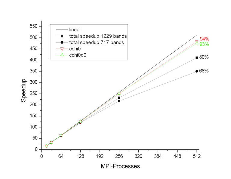
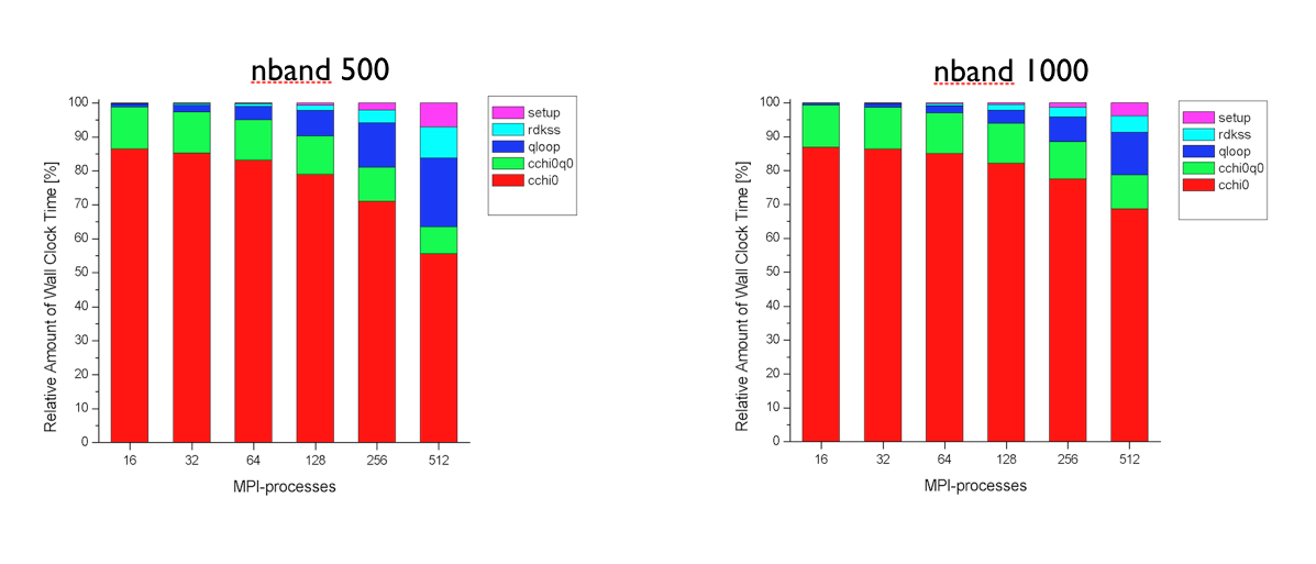
Tests performed at the Barcelona Supercomputing Center (see figures below) have revealed that the first and the second part of the MPI algorithm have a very good scaling. The routines cchi0 and cchi0q0 where the RPA expression is computed (step 1 and 2) scales almost linearly up to 512 processors. The degradation of the total speedup observed for large number of processors is mainly due to the portions of the computation that are not parallelized, namely the reading of the WFK file and the matrix inversion (qloop).
At this point, the most important technical details of the implementation have been covered, and we can finally run ABINIT over nn CPU cores using
(mpirun ...) abinit tmbt_2.abi > tmbt_2.log 2> err &
Run the input file tmb_2.abi using different number of processors and keep track of the time for each processor number so that we can test the scalability of the implementation. The performance analysis reported in the figures above was obtained with PAW using ZnO as tests case, but you should observe a similar behavior also in SiO2.
Now let us have a look at the output results. Since this tutorial mainly focuses on how to run efficient MPI computations, we will not perform any converge study for SiO2. Most of the parameters used in the input files are already close to converge, only the k-point sampling and the number of empty states should be increased. You might modify the input files to perform the standard converge tests following the procedure described in the first GW tutorial.
In the main output file, there is a section reporting how the bands are distributed among the nodes. For a sequential calculation, we have
 screening : taking advantage of time-reversal symmetry
 Maximum band index for partially occupied states nbvw =    24
 Remaining bands to be divided among processors   nbcw =    26
 Number of bands treated by each node ~   26
The value reported in the last line will decrease when the computation is done with more processors.
The memory allocated for the wavefunctions scales with the number of processors. You can use the grep utility to extract this information from the log file. For a calculation in sequential, we have:
>>> grep "Memory needed" tmbt_2.log

  Memory needed for storing ug=         29.5 [Mb]
  Memory needed for storing ur=        180.2 [Mb]
ug denotes the internal buffer used to store the Fourier components of the orbitals whose size scales linearly with %npwwfn. ur is the array storing the orbitals on the real space FFT mesh. Keep in mind that the size of ur scales linearly with the total number of points in the FFT box, number that is usually much larger than the number of planewaves (%npwwfn). The number of FFT divisions used in the GW code can be extracted from the main output file using
>>> grep setmesh tmbt_2.out  -A 1
 setmesh: FFT mesh size selected  =  27x 27x 36
          total number of points  =    26244
As discussed in this section of the GW notes, the Fast Fourier Transform represents one of the most CPU intensive part of the execution. For this reason the code provides the input variable fftgw that can be used to decrease the number of FFT points for better efficiency. The second digit of the input variable gwmem, instead, governs the storage of the real space orbitals and can used to avoid the storage of the costly array ur at the price of an increase in computational time.
2.d Manual parallelization over q-points.
The computational effort required by the screening computation scales linearly with the number of q-points. As explained in this section of the GW notes, the code exploits the symmetries of the screening function so that only the irreducible Brillouin zone (IBZ) has to be calculated explicitly. On the other hand, a large number of q-points might be needed to achieve converged results. Typical examples are GW calculations in metals or optical properties within the Bethe-Salpeter formalism.
If enough processing units are available, the linear factor due to the q-point sampling can be trivially absorbed by splitting the calculation of the q-points into several independent runs using the variables nqptdm and qptdm. The results can then be gathered in a unique binary file by means of the mrgscr utility (see also the automatic tests v3[87], v3[88] and v3[89]).
3 Computing the screening in parallel using the Hilbert transform method
As discussed in the GW_notes the algorithm based on the Adler-Wiser expression is not optimal when many frequencies are wanted. In this paragraph, we therefore discuss how to use the Hilbert transform method to calculate the RPA polarizability on a dense frequency mesh. The equations implemented in the code are documented in in this section.
As usual, we have to copy the file tmbt_3.abi in the working directory, and then create a symbolic link pointing to the WFK file.
>>> ln -s tmbt_1o_DS2_WFK tmbt_3i_WFK
The input file is $ABI_TESTS/tutoparal/Input/tmbt_3.abi. Open it so that we can have a look at its structure.
# Crystalline alpha-quartz
# DATASET 1 : Screening calculation
#
optdriver   3    # Screening run
irdwfk      1    # To read the WFK file.
symchi      1    # Use symmetries to speedup the BZ integration
ecutwfn     36   # Cutoff for the wavefunctions.
ecuteps     8    # Cutoff for the polarizability.
nband       50   # Number of bands in the spectral function (24 occupied bands).
inclvkb     2    # Correct treatment of the optical limit.

gwcalctyp   2    # Contour-deformation technique.
spmeth      1    # Enable the spectral method.
nomegasf  100    # Number of points for the spectral function.
gwpara      2    # Parallelization over bands
awtr        1    # Take advantage of time-reversal. Mandatory when gwpara=2 is used.
freqremax  40 eV # Frequency mesh for the polarizability
nfreqre    20
nfreqim     5

timopt -1

#################### COMMON PART #########################

# number of self-consistent field steps
nstep        200

# energy cutoff [Ha]:
ecut         36

#Definition of the k-point grid
occopt 1           # Semiconductor
kptopt 1           # Option for the automatic generation of k points, taking
                   # into account the symmetry

ngkpt   4 4 3
nshiftk  1
shiftk  0.0 0.0 0.0
istwfk  *1

# Definition of the atom types
npsp   2
znucl  14  8
ntypat 2

# Definition of the atoms
natom 9
typat 3*1  6*2

# Experimental parameters (Wyckoff pag 312)
# u(Si)= 0.465
# x= 0.415 ; y= 0.272 ; z= 0.120

acell   2*4.91304  5.40463  Angstrom

xred   0.465   0.000   0.000              #Si
       0.000   0.465   2/3                #Si
      -0.465  -0.465   1/3                #Si
       0.415   0.272   0.120              #O
      -0.143  -0.415   0.4533333333333333 #O
      -0.272   0.143   0.7866666666666666 #O
       0.143  -0.272  -0.120              #O
       0.272   0.415   0.5466666666666666 #O
      -0.415  -0.143   0.2133333333333333 #O

rprim   5.0000000000e-01 -8.6602540378e-01  0.0000000000e+00
        5.0000000000e-01  8.6602540378e-01  0.0000000000e+00
        0.0000000000e+00  0.0000000000e+00  1.0000000000e+00

 pp_dirpath "$ABI_PSPDIR"
 pseudos "Psdj_nc_sr_04_pw_std_psp8/Si.psp8, Psdj_nc_sr_04_pw_std_psp8/O.psp8"

##############################################################
# This section is used only for regression testing of ABINIT #
##############################################################
#%%<BEGIN TEST_INFO>
#%% [setup]
#%% executable = abinit
#%% test_chain = tmbt_1.abi, tmbt_2.abi, tmbt_3.abi
##%% test_chain = tmbt_1.abi, tmbt_2.abi, tmbt_3.abi, tmbt_4.abi
#%% [files]
#%% [paral_info]
#%% max_nprocs = 64
#%% nprocs_to_test = 64
#%% [NCPU_64]
#%% files_to_test = tmbt_3_MPI64.abo, tolnlines = 10, tolabs = 1.100e-03, tolrel = 3.000e-03
#%% [extra_info]
#%% authors = M. Giantomassi
#%% keywords =  GW
#%% description = GW calculation for crystalline alpha-quartz.
#%%   Screening calculation with Hilbert transform
#%%<END TEST_INFO>
A snapshot of the most important parameters governing the algorithm is reported below.
gwcalctyp   2    # Contour-deformation technique.
spmeth      1    # Enable the spectral method.
nomegasf  100    # Number of points for the spectral function.
gwpara      2    # Parallelization over bands
awtr        1    # Take advantage of time-reversal. Mandatory when gwpara=2 is used.
freqremax  40 eV # Frequency mesh for the polarizability
nfreqre    20
nfreqim     5
The input file is similar to the one we used for the Adler-Wiser calculation. The input variable spmeth enables the spectral method. nomegasf defines the number of ω′ points in the linear mesh used for the spectral function i.e. the number of ω′ in the equation for the spectral function.
As discussed in the [[theory:mbt#hilbert_transform|GW notes] for the spectral function. Hilbert transform method is much more memory demanding that the Adler-Wiser approach, mainly because of the large value of nomegasf that is usually needed to converge the results. Fortunately, the particular distribution of the data employed in gwpara = 2 turns out to be well suited for the calculation of the spectral function since each processor has to store and treat only a subset of the entire range of transition energies. The algorithm therefore presents good MPI-scalability since the number of ω′ frequencies that have to be stored and considered in the Hilbert transform decreases with the number of processors.
Now run ABINIT over nn CPU cores using
(mpirun ...) abinit tmbt_3.abi > tmbt_3.log 2> err
and test the scaling by varying the number of processors. Keep in mind that, also in this case, the distribution of the computing work is well balanced when the number of CPUs divides the number of conduction states.
The memory needed to store the spectral function is reported in the log file:
>>> grep "sf_chi0q0" tmbt_3.log
 memory required by sf_chi0q0:           1.0036 [Gb]
Note how the size of this array decreases when more processors are used.
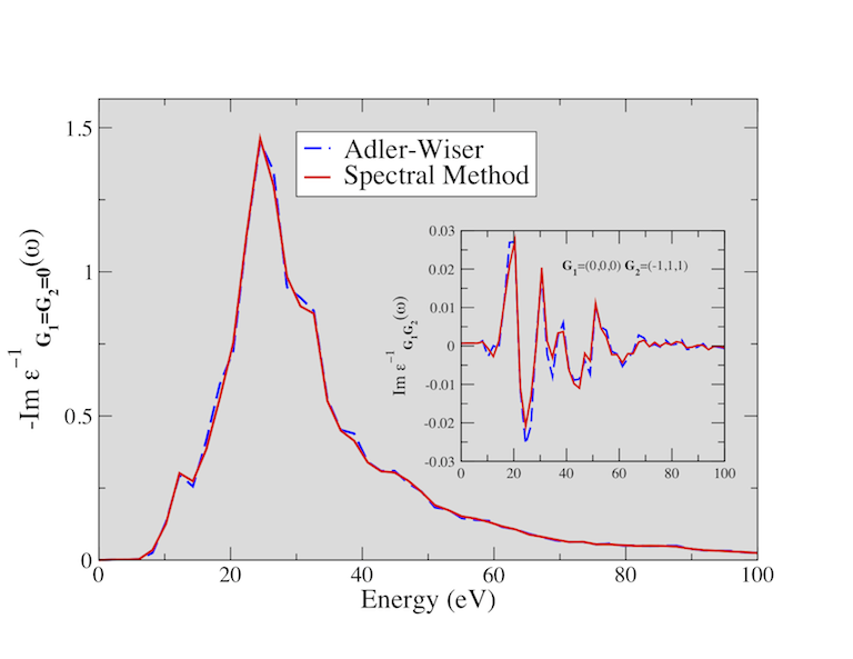
The figure below shows the electron energy loss function (EELF) of SiO2 calculated using the Adler-Wiser and the Hilbert transform method. You might try to reproduce these results (the EELF is reported in the file tmbt_3o_EELF, a much denser k-sampling is required to achieve convergence).
4 Computing the one-shot GW corrections in parallel
In this last paragraph, we discuss how to calculate G0W0 corrections in parallel with gwpara = 2. The basic equations used to compute the self-energy matrix elements are discussed in this part of the GW notes.
Before running the calculation, copy the file tmbt_4.abi in the working directory. Then create two symbolic links for the SCR and the WFK file:
ln -s tmbt_1o_DS2_WFK tmbt_4i_WFK
ln -s tmbt_2o_SCR     tmbt_4i_SCR
Now open the input file $ABI_TESTS/tutoparal/Input/tmbt_4.abi.
# Crystalline alpha-quartz
# DATASET 1 : Sigma calculation
#
optdriver   4            # Sigma run.
irdwfk      1
irdscr      1
gwcalctyp   0 ppmodel 1  # G0W0 calculation with the plasmon-pole approximation.
#gwcalctyp  2            # Uncomment this line to use the contour-deformation technique but remember to change the SCR file!
gwpara      2            # Parallelization over bands.
symsigma    1            # To enable the symmetrization of the self-energy matrix elements.
ecutwfn    36            # Cutoff for the wavefunctions.
ecuteps     8            # Cutoff in the correlation part.
ecutsigx   20            # Cutoff in the exchange part.
nband       50           # Number of bands for the correlation part.
gw_icutcoul   3            # old deprecated value of icutcoul, only used for legacy

timopt -1


# List of k-points for GW corrections.
nkptgw     5
kptgw
  0.00000000E+00  0.00000000E+00  0.00000000E+00
  2.50000000E-01  0.00000000E+00  0.00000000E+00
  5.00000000E-01  0.00000000E+00  0.00000000E+00
  2.50000000E-01  2.50000000E-01  0.00000000E+00
  0.00000000E+00  0.00000000E+00  3.33333333E-01
  2.50000000E-01  0.00000000E+00  3.33333333E-01
  5.00000000E-01  0.00000000E+00  3.33333333E-01
 -2.50000000E-01  0.00000000E+00  3.33333333E-01
  2.50000000E-01  2.50000000E-01  3.33333333E-01

bdgw
  24  25
  24  25
  24  25
  24  25
  24  25
  24  25
  24  25
  24  25
  24  25

#################### COMMON PART #########################

# number of self-consistent field steps
nstep        200

# energy cutoff [Ha]:
ecut         36

#Definition of the k-point grid
occopt 1           # Semiconductor
kptopt 1           # Option for the automatic generation of k points, taking
                   # into account the symmetry

ngkpt   4 4 3
nshiftk  1
shiftk  0.0 0.0 0.0
istwfk  *1

# Definition of the atom types
npsp   2
znucl  14  8
ntypat 2

# Definition of the atoms
natom 9
typat 3*1  6*2

# Experimental parameters (Wyckoff pag 312)
# u(Si)= 0.465
# x= 0.415 ; y= 0.272 ; z= 0.120

acell   2*4.91304  5.40463  Angstrom

xred   0.465   0.000   0.000              #Si
       0.000   0.465   2/3                #Si
      -0.465  -0.465   1/3                #Si
       0.415   0.272   0.120              #O
      -0.143  -0.415   0.4533333333333333 #O
      -0.272   0.143   0.7866666666666666 #O
       0.143  -0.272  -0.120              #O
       0.272   0.415   0.5466666666666666 #O
      -0.415  -0.143   0.2133333333333333 #O

rprim   5.0000000000e-01 -8.6602540378e-01  0.0000000000e+00
        5.0000000000e-01  8.6602540378e-01  0.0000000000e+00
        0.0000000000e+00  0.0000000000e+00  1.0000000000e+00

 pp_dirpath "$ABI_PSPDIR"
 pseudos "Psdj_nc_sr_04_pw_std_psp8/Si.psp8, Psdj_nc_sr_04_pw_std_psp8/O.psp8"

##############################################################
# This section is used only for regression testing of ABINIT #
##############################################################
#%%<BEGIN TEST_INFO>
#%% [setup]
#%% executable = abinit
#%% test_chain = tmbt_1.abi, tmbt_2.abi, tmbt_3.abi, tmbt_4.abi
#%% [files]
#%% [paral_info]
#%% max_nprocs = 64
#%% nprocs_to_test = 64
#%% [NCPU_64]
#%% files_to_test = tmbt_4_MPI64.abo, tolnlines = 0, tolabs = 0.0e+00, tolrel = 0.0e+00
#%% [extra_info]
#%% authors = M. Giantomassi
#%% keywords =  GW
#%% description = GW calculation for crystalline alpha-quartz. Sigma calculation
#%%<END TEST_INFO>
The most important parameters of the calculation are reported below:
optdriver   4            # Sigma run.
irdwfk      1
irdscr      1
gwcalctyp   0 ppmodel 1  # G<sub>0</sub>W<sub>0</sub> calculation with the plasmon-pole approximation.
#gwcalctyp  2            # Uncomment this line to use the contour-deformation technique but remember to change the SCR file!
gwpara      2            # Parallelization over bands.
symsigma    1            # To enable the symmetrization of the self-energy matrix elements.
ecutwfn    24            # Cutoff for the wavefunctions.
ecuteps     8            # Cutoff in the correlation part.
ecutsigx   20            # Cutoff in the exchange part.
nband       50           # Number of bands for the correlation part.
For our purposes, it suffices to say that this input file defines a standard one-shot calculation with the plasmon-pole model approximation. We refer to the documentation and to the first GW tutorial for a more complete description of the meaning of these variables.
Also in this case, we use gwpara = 2 to perform the calculation in parallel. Note, however, that the distribution of the orbitals employed in the self- energy part significantly differs from the one used to compute the screening. In what follows, we briefly describe the two-step procedure used to distribute the wavefunctions:
-
Each node reads and stores in memory the states where the QP corrections are computed (the list of states specified by kptgw and bdgw).
-
The nband bands are distributed using the following partition scheme:
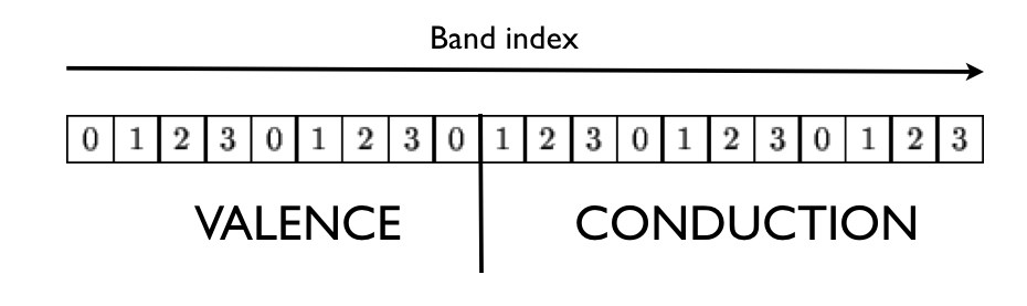
where we have assumed a calculation done with four nodes (the index in the box denotes the MPI rank).
By virtue of the particular distribution adopted, the computation of the correlation part is expected to scale well with the number CPUs. The maximum number of processors that can be used is limited by nband. Note, however, that only a subset of processors will receive the occupied states when the bands are distributed in step 2. As a consequence, the theoretical maximum speedup that can be obtained in the exchange part is limited by the availability of the occupied states on the different MPI nodes involved in the run.
The best-case scenario is when the QP corrections are wanted for all the occupied states. In this case, indeed, each node can compute part of the self- energy and almost linear scaling should be reached. The worst-case scenario is when the quasiparticle corrections are wanted only for a few states (e.g. band gap calculations) and NCPU >> Nvalence. In this case, indeed, only Nvalence processors will participate to the calculation of the exchange part.
To summarize: The MPI computation of the correlation part is efficient when the number of processors divides nband. Optimal scaling in the exchange part is obtained only when each node possesses the full set of occupied states.
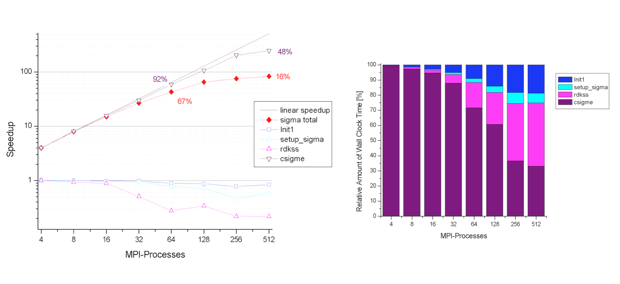
The two figures below show the speedup of the sigma part as function of the number of processors. The self-energy is calculated for 5 quasiparticle states using nband=1024 (205 occupied states). Note that this setup is close to the worst-case scenario. The computation of the self-energy matrix elements (csigme) scales well up to 64 processors. For large number number of CPUs, the scaling departs from the linear behavior due to the unbalanced distribution of the occupied bands. The non-scalable parts of the implementation (init1, rdkss) limit the total speedup due to Amdhal’s law.
The implementation presents good memory scalability since the largest arrays are distributed. Only the size of the screening does not scale with the number of nodes. By default each CPU stores in memory the entire screening matrix for all the q-points and frequencies in order to optimize the computation. In the case of large matrices, however, it possible to opt for an out-of-core solution in which only a single q-point is stored in memory and the data is read from the external SCR file (slower but less memory demanding). This option is controlled by the first digit of gwmem.
Now that we know how distribute the load efficiently, we can finally run the calculation using
(mpirun ...) abinit tmbt_4.abi > tmbt_4.log 2> err &
Keep track of the time for each processor number so that we can test the scalability of the self-energy part.
Please note that the results of these tests are not converged. A well converged calculation would require a 6x6x6 k-mesh to sample the full BZ, and a cutoff energy of 10 Ha for the screening matrix. The QP results converge extremely slowly with respect to the number of empty states. To converge the QP gaps within 0.1 eV accuracy, we had to include 1200 bands in the screening and 800 states in the calculation of the self-energy.
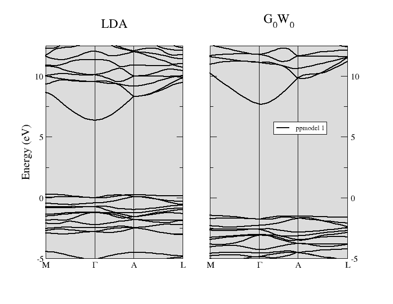
The comparison between the LDA band structure and the G0W0 energy bands of α-quartz SiO2 is reported in the figure below. The direct gap at Γ is opened up significantly from the LDA value of 6.1 eV to about 9.4 eV when the one- shot G0W0 method is used. You are invited to reproduce this result (take into account that this calculation has been performed at the theoretical LDA parameters, while the experimental structure is used in all the input files of this tutorial).
5 Basic rules for efficient parallel calculations
-
Remember that “Anything that can possibly go wrong, does”. So, when writing your input file, try to “Keep It Short and Simple”.
-
Do one thing and do it well: Avoid using different values of optdriver in the same input file. Each runlevel employs different approaches to distribute memory and CPU time, hence it is almost impossible to find the number of processors that will produce a balanced run in each dataset.
-
Prime number theorem: Convergence studies should be executed in parallel only when the parameters that are tested do not interfere with the MPI algorithm. For example, the convergence study in the number of bands in the screening should be done in separated input files when gwpara=2 is used.
-
Less is more: Split big calculations into smaller runs whenever possible. For example, screening calculations can be split over q-points. The calculation of the self-energy can be easily split over kptgw and bdgw.
-
Look before you leap: Use the converge tests to estimate how the CPU-time and the memory requirements depend on the parameter that is tested. Having an estimate of the computing resources is very helpful when one has to launch the final calculation with converged parameters.