First tutorial
The H2 molecule without convergence studies
This tutorial aims at showing how to get the following physical properties:
- the (pseudo) total energy
- the bond length
- the charge density
- the atomisation energy
You will learn about the two input files, the basic input variables, the existence of defaults, the actions of the parser, and the use of the multi-dataset feature. You will also learn about the two output files as well as the density file.
This first tutorial covers the first sections of the abinit help file. The very first step is a detailed tour of the input and output files: you are like a tourist, and you discover a town in a coach. You will have a bit more freedom after that first step. It is supposed that you have some good knowledge of UNIX/Linux.
Visualisation tools are NOT covered in the basic ABINIT tutorials. Powerful visualisation procedures have been developed in the Abipy context, relying on matplotlib. See the README of Abipy and the Abipy tutorials.
This tutorial should take about 2 hours.
Note
Supposing you made your own installation of ABINIT, the input files to run the examples are in the ~abinit/tests/ directory where ~abinit is the absolute path of the abinit top-level directory. If you have NOT made your own install, ask your system administrator where to find the package, especially the executable and test files.
In case you work on your own PC or workstation, to make things easier, we suggest you define some handy environment variables by executing the following lines in the terminal:
export ABI_HOME=Replace_with_absolute_path_to_abinit_top_level_dir # Change this line
export PATH=$ABI_HOME/src/98_main/:$PATH      # Do not change this line: path to executable
export ABI_TESTS=$ABI_HOME/tests/             # Do not change this line: path to tests dir
export ABI_PSPDIR=$ABI_TESTS/Pspdir/  # Do not change this line: path to pseudos dir
Examples in this tutorial use these shell variables: copy and paste
the code snippets into the terminal (remember to set ABI_HOME first!) or, alternatively,
source the set_abienv.sh script located in the ~abinit directory:
source ~abinit/set_abienv.sh
The ‘export PATH’ line adds the directory containing the executables to your PATH so that you can invoke the code by simply typing abinit in the terminal instead of providing the absolute path.
To execute the tutorials, create a working directory (Work*) and
copy there the input files of the lesson.
Most of the tutorials do not rely on parallelism (except specific tutorials on parallelism). However you can run most of the tutorial examples in parallel with MPI, see the topic on parallelism.
Computing the (pseudo) total energy and some associated quantities
For this tutorial, one needs a working directory. So, you should create a Work subdirectory inside $ABI_TESTS/tutorial, e.g. with the commands:
cd $ABI_TESTS/tutorial/Input
mkdir Work   # ~abinit/tests/tutorial/Input/Work
cd Work
We will do most of the actions of this tutorial in this working directory. Let us now run the code …
Tip
The section 1.1 of the ABINIT help file explains how to run ABINIT. You might read it now, then follow the commands hereafter.
Copy $ABI_TESTS/tutorial/Input/tbase1_1.abi in Work:
cp ../tbase1_1.abi .
Later, we will look at this file, and learn about its content. For now, you will try to run the code. In the Work directory, type:
abinit tbase1_1.abi >& log &
Wait a few seconds … it’s done! You can look at the content of the Work directory with the ls command. You should get something like:
ls
log           tbase1_1o_DDB     tbase1_1o_EIG     tbase1_1o_OUT.nc
tbase1_1.abi  tbase1_1o_DEN     tbase1_1o_EIG.nc  tbase1_1o_WFK
tbase1_1.abo  tbase1_1o_EBANDS.agr  tbase1_1o_GSR.nc
Different output files have been created, including a log file and the output file tbase1_1.abo. To check that everything is correct, you can make a diff of tbase1_1.abo with the reference file $ABI_TESTS/tutorial/Refs/tbase1_1.abo
diff tbase1_1.abo ../../Refs/tbase1_1.abo | less
That reference file uses slightly different file names. You should get some difference, but rather inoffensive ones, like differences in the name of input files, slightly different numerical results, or timing differences, e.g.:
2,3c2,3
< .Version 9.4.1 of ABINIT
< .(MPI version, prepared for a x86_64_darwin18.7.0_gnu9.3 computer)
---
> .Version 9.3.3 of ABINIT
> .(MPI version, prepared for a x86_64_linux_gnu9.3 computer)
17,18c17,18
< .Starting date : Mon 25 Jan 2021.
< - ( at 21h07 )
---
> .Starting date : Wed 30 Dec 2020.
> - ( at 19h15 )
20,21c20,21
< - input  file    -> tbase1_1.abi
< - output file    -> tbase1_1.abo
---
> - input  file    -> /home/buildbot/ABINIT/alps_gnu_9.3_serial/trunk_beauty/tests/TestBot_MPI1/tutorial_tbase1_1/tbase1_1.abi
> - output file    -> tbase1_1.abo
117,118c117,118
< - pspini: atom type   1  psp file is /Users/gonze/_Research/ABINIT_git/beauty/tests/Pspdir/Pseudodojo_nc_sr_04_pw_standard_psp8/H.psp8
< - pspatm: opening atomic psp file    /Users/gonze/_Research/ABINIT_git/beauty/tests/Pspdir/Pseudodojo_nc_sr_04_pw_standard_psp8/H.psp8
---
> - pspini: atom type   1  psp file is /home/buildbot/ABINIT/alps_gnu_9.3_openmpi/trunk_beauty/tests/Pspdir/Pseudodojo_nc_sr_04_pw_standard_psp8/H.psp8
> - pspatm: opening atomic psp file    /home/buildbot/ABINIT/alps_gnu_9.3_openmpi/trunk_beauty/tests/Pspdir/Pseudodojo_nc_sr_04_pw_standard_psp8/H.psp8
216,217c216,217
<     1     -1.38336201933863    -0.00000000000000    -0.00000000000000
<     2      1.38336201933863    -0.00000000000000    -0.00000000000000
---
>     1     -1.38336201933879    -0.00000000000000    -0.00000000000000
>     2      1.38336201933879    -0.00000000000000    -0.00000000000000
230,232c230,232
< kinetic             :  1.01705426532945E+00
< hartree             :  7.26359620833820E-01
< xc                  : -6.39065298290653E-01
---
> kinetic             :  1.01705426532942E+00
> hartree             :  7.26359620833802E-01
> xc                  : -6.39065298290642E-01
239c239
< band_energy         : -7.38843481479430E-01
---
> band_energy         : -7.38843481479398E-01
314c314
< - Total cpu        time (s,m,h):          4.7        0.08      0.001
---
> - Total cpu        time (s,m,h):          4.6        0.08      0.001
321,329c321,328
If you do not run on a PC under Linux with GNU Fortran compiler, e.g. the Intel compiler, you might also have small numerical differences, on the order of 1.0d-10 at most. You might also have other differences in the paths of files. Finally, it might also be that the default FFT algorithm differs from the one of the reference machine, in which case the line mentioning fftalg will differ (fftalg will not be 312). If you get something else, you should ask for help!
You can have a very quick look at the beginning of the output file tbase1_1.abo.
In this part of the output file, note the dot . or dash - that is inserted in the first column.
This is not important for the user: it is used to post-process the output file using some automatic tool.
As a rule, you should ignore symbols placed in the first column of the abinit output file.
Supposing everything went well, we will now detail the different steps that took place: how to run the code, what is in the tbase1_1.abi input file, and, later, what is in the tbase1_1.abo and log output files.
Tip
If you have not read it, please read section 1.1 of the ABINIT help file.
It is now time to edit the tbase1_1.abi input file.
# H2 molecule in a big box
#
# In this input file, the location of the information on this or that line
# is not important : a keyword is located by the parser, and the related
# information should follow. Still, this file is strongly structured, for pedagogical purpose.
# The "#" symbol indicates the beginning of a comment : the remaining
# of the line will be skipped.

#Definition of the unit cell
acell 10 10 10    # The keyword "acell" refers to the
                  # lengths of the primitive vectors (in Bohr)
#rprim 1 0 0  0 1 0  0 0 1 # This line, defining orthogonal primitive vectors,
                           # is commented, because it is precisely the default value of rprim

#Definition of the atom types and pseudopotentials
ntypat 1          # There is only one type of atom
znucl 1           # The keyword "znucl" refers to the atomic number of the possible type(s) of atom.
                  # Here, the only type is Hydrogen. The pseudopotential(s)
                  # mentioned after the keyword "pseudos" should correspond to this type of atom.
pp_dirpath "$ABI_PSPDIR"                 # This is the path to the directory were pseudopotentials for tests are stored
pseudos "Psdj_nc_sr_04_pw_std_psp8/H.psp8"  # Name and location of the pseudopotential
                  # This pseudopotential comes from the pseudodojo site http://www.pseudo-dojo.org/  (NC SR LDA standard),
                  # and was generated using the LDA exchange-correlation functional (PW=Perdew-Wang, ixc=-1012).
                  # By default, abinit uses the same exchange-correlation functional than the one of the input pseudopotential(s)

#Definition of the atoms
natom 2           # There are two atoms
typat 1 1         # They both are of type 1, that is, Hydrogen
xcart             # This keyword indicates that the location of the atoms
                  # will follow, one triplet of number for each atom
  -0.7 0.0 0.0    # Triplet giving the cartesian coordinates of atom 1, in Bohr
   0.7 0.0 0.0    # Triplet giving the cartesian coordinates of atom 2, in Bohr

#Numerical parameters of the calculation : planewave basis set and k point grid
ecut 10.0         # Maximal plane-wave kinetic energy cut-off, in Hartree
kptopt 0          # Enter the k points manually
nkpt 1            # Only one k point is needed for isolated system,
                  # taken by default to be 0.0 0.0 0.0

#Parameters for the SCF procedure
nstep 10          # Maximal number of SCF cycles
toldfe 1.0d-6     # Will stop when, twice in a row, the difference
                  # between two consecutive evaluations of total energy
                  # differ by less than toldfe (in Hartree)
                  # This value is way too large for most realistic studies of materials
diemac 2.0        # Although this is not mandatory, it is worth to
                  # precondition the SCF cycle. The model dielectric
                  # function used as the standard preconditioner
                  # is described in the "dielng" input variable section.
                  # Here, we follow the prescriptions for molecules in a big box

##############################################################
# This section is used only for regression testing of ABINIT #
##############################################################
#%%<BEGIN TEST_INFO>
#%% [setup]
#%% executable = abinit
#%% [files]
#%% files_to_test =
#%%   tbase1_1.abo, tolnlines=  0, tolabs=  0.000e+00, tolrel=  0.000e+00
#%% [paral_info]
#%% max_nprocs = 1
#%% [extra_info]
#%% authors = X. Gonze
#%% keywords =
#%% description = H2 molecule in a big box
#%%<END TEST_INFO>
You can have a first glance at it. It is not very long: about 50 lines, mostly comments. Do not try to understand everything immediately. After having gone through it, you should read general explanation about its content, and the format of such input files in the section 3.1 of the abinit help file.
You might now examine in more details some input variables. An alphabetically ordered index of all variables is provided, and their description is found in different files (non-exhaustive list):
- Basic variables
- Files handling variables
- Ground-state calculation variables
- GW variables
- Parallelisation variables
- Density Functional Perturbation Theory (DFPT) variables
However, the number of such variables is rather large! Note that only a dozen of input variables were needed to run the first test case. This is possible because there are defaults values for the other input variables. When it exists, the default value is mentioned at the fourth line of the section related to each input variable. Some input variables are also preprocessed, in order to derive convenient values for other input variables. Defaults are not existing or were avoided for the few input variables that you find in tbase1_1.abi. These are particularly important input variables. So, take a few minutes to have a look at the input variables of tbase1_1.abi:
Have also a look at kpt and iscf.
It is now time to have a look at the two output files of the run.
First, open the log file. You can begin to read it. It is nasty. Jump to its end. Twenty lines before the end, you will find the number of WARNINGS and COMMENTS that were issued by the code during execution. You might try to find them in the file (localize the keywords WARNING or COMMENT in this file). Some of them are for the experienced user. For the present time, we will ignore them. You can find more information about messages in the log file in this section of the abinit help file.
Tip
If AbiPy is installed on your machine, you can use the abiopen.py script to extract the messages from the Abinit log file with the syntax:
abiopen.py log -p
to get:
Events found in /Users/gonze/_Research/ABINIT_git/beauty/tests/tutorial/Input/Work/log

[1] <AbinitComment at m_dtfil.F90:1470>
    Output file: tbase1_1.abo already exists.

[2] <AbinitComment at m_dtfil.F90:1494>
    Renaming old: tbase1_1.abo to: tbase1_1.abo0001

[3] <AbinitWarning at m_ingeo.F90:887>
    The tolerance on symmetries =   1.000E-05 is bigger than 1.0e-8.
    In order to avoid spurious effects, the atomic coordinates have been
    symmetrized before storing them in the dataset internal variable.
    So, do not be surprised by the fact that your input variables (xcart, xred, ...)
    do not correspond to the ones echoed by ABINIT, the latter being used to do the calculations.
    In order to avoid this symmetrization (e.g. for specific debugging/development), decrease tolsym to 1.0e-8 or lower.

[4] <AbinitComment at m_symfind.F90:999>
    The Bravais lattice determined only from the primitive
    vectors, bravais(1)=  7, is more symmetric
    than the real one, iholohedry=  4, obtained by taking into
    account the atomic positions. Start deforming the primitive vector set.

[5] <AbinitComment at m_memeval.F90:2397>
    Despite there is only a local part to pseudopotential(s),
    lmnmax and lnmax are set to 1.

[6] <AbinitComment at m_xgScalapack.F90:236>
    xgScalapack in auto mode

[7] <AbinitComment at m_memeval.F90:2397>
    Despite there is only a local part to pseudopotential(s),
    lmnmax and lnmax are set to 1.

[8] <AbinitWarning at m_drivexc.F90:711>
    Density went too small (lower than xc_denpos) at 38 points
    and was set to xc_denpos =   1.00E-14. Lowest was  -0.13E-13.
    This might be due to (1) too low boxcut or (2) too low ecut for
    pseudopotential core charge, or (3) too low ecut for estimated initial density.
    Possible workarounds : increase ecut, or define the input variable densty,
    with a value larger than the guess for the decay length, or initialize your,
    density with a preliminary LDA or GGA-PBE if you are using a more exotic xc functional.

num_errors: 0, num_warnings: 2, num_comments: 6, completed: True
Now open the tbase1_1.abo file. Alternatively, you might have a look at the reference file we provide below.
.Version 10.5.8.2 of ABINIT, released Oct 2025.
.(MPI version, prepared for a x86_64_linux_gnu13.2 computer)

.Copyright (C) 1998-2026 ABINIT group .
 ABINIT comes with ABSOLUTELY NO WARRANTY.
 It is free software, and you are welcome to redistribute it
 under certain conditions (GNU General Public License,
 see ~abinit/COPYING or http://www.gnu.org/copyleft/gpl.txt).

 ABINIT is a project of the Universite Catholique de Louvain,
 Corning Inc. and other collaborators, see ~abinit/doc/developers/contributors.txt .
 Please read https://docs.abinit.org/theory/acknowledgments for suggested
 acknowledgments of the ABINIT effort.
 For more information, see https://www.abinit.org .

.Starting date : Sat 20 Dec 2025.
- ( at 17h05 )

- input  file    -> /home/buildbot/ABINIT3/eos_gnu_13.2_mpich/trunk__codata2022/tests/TestBot_MPI1/tutorial_tbase1_1/tbase1_1.abi
- output file    -> tbase1_1.abo
- root for input  files -> tbase1_1i
- root for output files -> tbase1_1o

 Symmetries : space group P4/m m m (#123); Bravais tP (primitive tetrag.)
================================================================================
 Values of the parameters that define the memory need of the present run
     intxc =       0    ionmov =       0      iscf =       7    lmnmax =       3
     lnmax =       3     mgfft =      30  mpssoang =       2    mqgrid =    3001
     natom =       2  nloc_mem =       1    nspden =       1   nspinor =       1
    nsppol =       1      nsym =      16    n1xccc =       0    ntypat =       1
    occopt =       1   xclevel =       1
-    mband =           2        mffmem =           1         mkmem =           1
       mpw =         752          nfft =       27000          nkpt =           1
================================================================================
P This job should need less than                       8.712 Mbytes of memory.
  Rough estimation (10% accuracy) of disk space for files :
_ WF disk file :      0.025 Mbytes ; DEN or POT disk file :      0.208 Mbytes.
================================================================================

--------------------------------------------------------------------------------
------------- Echo of variables that govern the present computation ------------
--------------------------------------------------------------------------------
-
- outvars: echo of selected default values
-   iomode0 =  0 , fftalg0 =512 , wfoptalg0 =  0
-
- outvars: echo of global parameters not present in the input file
-  max_nthreads =    0
-
 -outvars: echo values of preprocessed input variables --------
            acell      1.0000000000E+01  1.0000000000E+01  1.0000000000E+01 Bohr
              amu      1.00794000E+00
           diemac      2.00000000E+00
             ecut      1.00000000E+01 Hartree
-          fftalg         512
           istwfk        2
              ixc       -1012
           kptopt           0
P           mkmem           1
            natom           2
            nband           2
            ngfft          30      30      30
             nkpt           1
            nstep          10
             nsym          16
           ntypat           1
              occ      2.000000  0.000000
          spgroup         123
           symrel      1  0  0   0  1  0   0  0  1      -1  0  0   0 -1  0   0  0 -1
                      -1  0  0   0  1  0   0  0 -1       1  0  0   0 -1  0   0  0  1
                      -1  0  0   0 -1  0   0  0  1       1  0  0   0  1  0   0  0 -1
                       1  0  0   0 -1  0   0  0 -1      -1  0  0   0  1  0   0  0  1
                       1  0  0   0  0  1   0  1  0      -1  0  0   0  0 -1   0 -1  0
                      -1  0  0   0  0  1   0 -1  0       1  0  0   0  0 -1   0  1  0
                      -1  0  0   0  0 -1   0  1  0       1  0  0   0  0  1   0 -1  0
                       1  0  0   0  0 -1   0 -1  0      -1  0  0   0  0  1   0  1  0
           toldfe      1.00000000E-06 Hartree
            typat      1  1
           xangst     -3.7042404738E-01  0.0000000000E+00  0.0000000000E+00
                       3.7042404738E-01  0.0000000000E+00  0.0000000000E+00
            xcart     -7.0000000000E-01  0.0000000000E+00  0.0000000000E+00
                       7.0000000000E-01  0.0000000000E+00  0.0000000000E+00
             xred     -7.0000000000E-02  0.0000000000E+00  0.0000000000E+00
                       7.0000000000E-02  0.0000000000E+00  0.0000000000E+00
            znucl        1.00000

================================================================================

 chkinp: Checking input parameters for consistency.

================================================================================
== DATASET  1 ==================================================================
-   mpi_nproc: 1, omp_nthreads: -1 (-1 if OMP is not activated)


--- !DatasetInfo
iteration_state: {dtset: 1, }
dimensions: {natom: 2, nkpt: 1, mband: 2, nsppol: 1, nspinor: 1, nspden: 1, mpw: 752, }
cutoff_energies: {ecut:  10.0, pawecutdg:  -1.0, }
electrons: {nelect:   2.00000000E+00, charge:   0.00000000E+00, occopt:   1.00000000E+00, tsmear:   1.00000000E-02, }
meta: {optdriver: 0, ionmov: 0, optcell: 0, iscf: 7, paral_kgb: 0, }
...

 Real(R)+Recip(G) space primitive vectors, cartesian coordinates (Bohr,Bohr^-1):
 R(1)= 10.0000000  0.0000000  0.0000000  G(1)=  0.1000000  0.0000000  0.0000000
 R(2)=  0.0000000 10.0000000  0.0000000  G(2)=  0.0000000  0.1000000  0.0000000
 R(3)=  0.0000000  0.0000000 10.0000000  G(3)=  0.0000000  0.0000000  0.1000000
 Unit cell volume ucvol=  1.0000000E+03 bohr^3
 Angles (23,13,12)=  9.00000000E+01  9.00000000E+01  9.00000000E+01 degrees

 getcut: wavevector=  0.0000  0.0000  0.0000  ngfft=  30  30  30
         ecut(hartree)=     10.000   => boxcut(ratio)=   2.10744

--- Pseudopotential description ------------------------------------------------
- pspini: atom type   1  psp file is /home/buildbot/ABINIT3/eos_gnu_13.2_mpich/trunk__codata2022/tests/Pspdir/Psdj_nc_sr_04_pw_std_psp8/H.psp8
- pspatm: opening atomic psp file    /home/buildbot/ABINIT3/eos_gnu_13.2_mpich/trunk__codata2022/tests/Pspdir/Psdj_nc_sr_04_pw_std_psp8/H.psp8
- H     ONCVPSP-3.3.0  r_core=   1.00957   0.90680
-  1.00000   1.00000    171101                znucl, zion, pspdat
    8   -1012    1    4       300   0.00000   pspcod,pspxc,lmax,lloc,mmax,r2well
    2.99000000000000    0.00000000000000    0.00000000000000   rchrg,fchrg,qchrg
     nproj     2     1
     extension_switch     1
  pspatm : epsatm=    0.35491505
         --- l  ekb(1:nproj) -->
             0   -1.665338   -0.519510
             1   -0.275071
 pspatm: atomic psp has been read  and splines computed

   1.41966018E+00                                ecore*ucvol(ha*bohr**3)
--------------------------------------------------------------------------------

_setup2: Arith. and geom. avg. npw (full set) are    1503.000    1503.000

================================================================================

--- !BeginCycle
iteration_state: {dtset: 1, }
solver: {iscf: 7, nstep: 10, nline: 4, wfoptalg: 0, }
tolerances: {toldfe: 1.00E-06, }
...

     iter   Etot(hartree)      deltaE(h)  residm     vres2
 ETOT  1  -1.1093804698962    -1.109E+00 6.384E-04 1.736E+01
 ETOT  2  -1.1170431098364    -7.663E-03 7.449E-08 2.737E-01
 ETOT  3  -1.1171736936408    -1.306E-04 5.867E-06 6.992E-02
 ETOT  4  -1.1171842773283    -1.058E-05 8.862E-07 5.492E-04
 ETOT  5  -1.1171843458762    -6.855E-08 1.683E-09 1.404E-05
 ETOT  6  -1.1171843463443    -4.681E-10 2.580E-11 3.672E-07

 At SCF step    6, etot is converged :
  for the second time, diff in etot=  4.681E-10 < toldfe=  1.000E-06

 Cartesian components of stress tensor (hartree/bohr^3)
  sigma(1 1)= -3.33791900E-06  sigma(3 2)=  0.00000000E+00
  sigma(2 2)=  3.45795063E-05  sigma(3 1)=  0.00000000E+00
  sigma(3 3)=  3.45795063E-05  sigma(2 1)=  0.00000000E+00


--- !ResultsGS
iteration_state: {dtset: 1, }
comment   : Summary of ground state results
lattice_vectors:
- [ 10.0000000,   0.0000000,   0.0000000, ]
- [  0.0000000,  10.0000000,   0.0000000, ]
- [  0.0000000,   0.0000000,  10.0000000, ]
lattice_lengths: [  10.00000,   10.00000,   10.00000, ]
lattice_angles: [ 90.000,  90.000,  90.000, ] # degrees, (23, 13, 12)
lattice_volume:   1.0000000E+03
convergence: {deltae: -4.681E-10, res2:  3.672E-07, residm:  2.580E-11, diffor: null, }
etotal    :  -1.11718435E+00
entropy   :   0.00000000E+00
fermie    :  -3.69421741E-01
cartesian_stress_tensor: # hartree/bohr^3
- [ -3.33791900E-06,   0.00000000E+00,   0.00000000E+00, ]
- [  0.00000000E+00,   3.45795063E-05,   0.00000000E+00, ]
- [  0.00000000E+00,   0.00000000E+00,   3.45795063E-05, ]
pressure_GPa:  -6.4551E-01
xred      :
- [ -7.0000E-02,   0.0000E+00,   0.0000E+00,  H]
- [  7.0000E-02,   0.0000E+00,   0.0000E+00,  H]
cartesian_forces: # hartree/bohr
- [ -2.69021104E-02,  -0.00000000E+00,  -0.00000000E+00, ]
- [  2.69021104E-02,  -0.00000000E+00,  -0.00000000E+00, ]
force_length_stats: {min:   2.69021104E-02, max:   2.69021104E-02, mean:   2.69021104E-02, }
...

 Integrated electronic density in atomic spheres:
 ------------------------------------------------
 Atom  Sphere_radius  Integrated_density
    1        2.00000          1.44870285
    2        2.00000          1.44870285
================================================================================

 ----iterations are completed or convergence reached----

 Mean square residual over all n,k,spin=   25.224E-12; max=  25.802E-12
 reduced coordinates (array xred) for    2 atoms
      -0.070000000000      0.000000000000      0.000000000000
       0.070000000000      0.000000000000      0.000000000000
 rms dE/dt=  1.5532E-01; max dE/dt=  2.6902E-01; dE/dt below (all hartree)
    1       0.269021103678      0.000000000000      0.000000000000
    2      -0.269021103678      0.000000000000      0.000000000000

 cartesian coordinates (angstrom) at end:
    1     -0.37042404738080     0.00000000000000     0.00000000000000
    2      0.37042404738080     0.00000000000000     0.00000000000000

 cartesian forces (hartree/bohr) at end:
    1     -0.02690211036782    -0.00000000000000    -0.00000000000000
    2      0.02690211036782    -0.00000000000000    -0.00000000000000
 frms,max,avg= 1.5531941E-02 2.6902110E-02   0.000E+00  0.000E+00  0.000E+00 h/b

 cartesian forces (eV/Angstrom) at end:
    1     -1.38336213552785    -0.00000000000000    -0.00000000000000
    2      1.38336213552785    -0.00000000000000    -0.00000000000000
 frms,max,avg= 7.9868450E-01 1.3833621E+00   0.000E+00  0.000E+00  0.000E+00 e/A
 length scales= 10.000000000000 10.000000000000 10.000000000000 bohr
              =  5.291772105440  5.291772105440  5.291772105440 angstroms
 prteigrs : about to open file tbase1_1o_EIG
 Fermi (or HOMO) energy (hartree) =  -0.36942   Average Vxc (hartree)=  -0.07352
 Eigenvalues (hartree) for nkpt=   1  k points:
 kpt#   1, nband=  2, wtk=  1.00000, kpt=  0.0000  0.0000  0.0000 (reduced coord)
  -0.36942   -0.01446

--- !EnergyTerms
iteration_state     : {dtset: 1, }
comment             : Components of total free energy in Hartree
kinetic             :  1.01705426532946E+00
hartree             :  7.26359620833829E-01
xc                  : -6.39065298290654E-01
Ewald energy        :  1.51051118525613E-01
psp_core            :  1.41966018330111E-03
local_psp           : -2.21187993697866E+00
non_local_psp       : -1.62123775947208E-01
total_energy        : -1.11718434634432E+00
total_energy_eV     : -3.04001347563390E+01
band_energy         : -7.38843481479434E-01
...


 Cartesian components of stress tensor (hartree/bohr^3)
  sigma(1 1)= -3.33791900E-06  sigma(3 2)=  0.00000000E+00
  sigma(2 2)=  3.45795063E-05  sigma(3 1)=  0.00000000E+00
  sigma(3 3)=  3.45795063E-05  sigma(2 1)=  0.00000000E+00

-Cartesian components of stress tensor (GPa)         [Pressure= -6.4551E-01 GPa]
- sigma(1 1)= -9.82049674E-02  sigma(3 2)=  0.00000000E+00
- sigma(2 2)=  1.01736420E+00  sigma(3 1)=  0.00000000E+00
- sigma(3 3)=  1.01736420E+00  sigma(2 1)=  0.00000000E+00

== END DATASET(S) ==============================================================
================================================================================

 -outvars: echo values of variables after computation  --------
            acell      1.0000000000E+01  1.0000000000E+01  1.0000000000E+01 Bohr
              amu      1.00794000E+00
           diemac      2.00000000E+00
             ecut      1.00000000E+01 Hartree
           etotal     -1.1171843463E+00
            fcart     -2.6902110368E-02 -0.0000000000E+00 -0.0000000000E+00
                       2.6902110368E-02 -0.0000000000E+00 -0.0000000000E+00
-          fftalg         512
           istwfk        2
              ixc       -1012
           kptopt           0
P           mkmem           1
            natom           2
            nband           2
            ngfft          30      30      30
             nkpt           1
            nstep          10
             nsym          16
           ntypat           1
              occ      2.000000  0.000000
          spgroup         123
           strten     -3.3379189980E-06  3.4579506319E-05  3.4579506319E-05
                       0.0000000000E+00  0.0000000000E+00  0.0000000000E+00
           symrel      1  0  0   0  1  0   0  0  1      -1  0  0   0 -1  0   0  0 -1
                      -1  0  0   0  1  0   0  0 -1       1  0  0   0 -1  0   0  0  1
                      -1  0  0   0 -1  0   0  0  1       1  0  0   0  1  0   0  0 -1
                       1  0  0   0 -1  0   0  0 -1      -1  0  0   0  1  0   0  0  1
                       1  0  0   0  0  1   0  1  0      -1  0  0   0  0 -1   0 -1  0
                      -1  0  0   0  0  1   0 -1  0       1  0  0   0  0 -1   0  1  0
                      -1  0  0   0  0 -1   0  1  0       1  0  0   0  0  1   0 -1  0
                       1  0  0   0  0 -1   0 -1  0      -1  0  0   0  0  1   0  1  0
           toldfe      1.00000000E-06 Hartree
            typat      1  1
           xangst     -3.7042404738E-01  0.0000000000E+00  0.0000000000E+00
                       3.7042404738E-01  0.0000000000E+00  0.0000000000E+00
            xcart     -7.0000000000E-01  0.0000000000E+00  0.0000000000E+00
                       7.0000000000E-01  0.0000000000E+00  0.0000000000E+00
             xred     -7.0000000000E-02  0.0000000000E+00  0.0000000000E+00
                       7.0000000000E-02  0.0000000000E+00  0.0000000000E+00
            znucl        1.00000

================================================================================


- Timing analysis has been suppressed with timopt=0


================================================================================

 Suggested references for the acknowledgment of ABINIT usage.

 The users of ABINIT have little formal obligations with respect to the ABINIT group
 (those specified in the GNU General Public License, http://www.gnu.org/copyleft/gpl.txt).
 However, it is common practice in the scientific literature,
 to acknowledge the efforts of people that have made the research possible.
 In this spirit, please find below suggested citations of work written by ABINIT developers,
 corresponding to implementations inside of ABINIT that you have used in the present run.
 Note also that it will be of great value to readers of publications presenting these results,
 to read papers enabling them to understand the theoretical formalism and details
 of the ABINIT implementation.
 For information on why they are suggested, see also https://docs.abinit.org/theory/acknowledgments.
-
- [1] Libxc: A library of exchange and correlation functionals for density functional theory.
- M.A.L. Marques, M.J.T. Oliveira, T. Burnus, Computer Physics Communications 183, 2227 (2012).
- Comment: to be cited when LibXC is used (negative value of ixc)
- Strong suggestion to cite this paper.
- DOI and bibtex: see https://docs.abinit.org/theory/bibliography/#marques2012
-
- [2] The Abinit project: Impact, environment and recent developments.
- Computer Phys. Comm. 248, 107042 (2020).
- X.Gonze, B. Amadon, G. Antonius, F.Arnardi, L.Baguet, J.-M.Beuken,
- J.Bieder, F.Bottin, J.Bouchet, E.Bousquet, N.Brouwer, F.Bruneval,
- G.Brunin, T.Cavignac, J.-B. Charraud, Wei Chen, M.Cote, S.Cottenier,
- J.Denier, G.Geneste, Ph.Ghosez, M.Giantomassi, Y.Gillet, O.Gingras,
- D.R.Hamann, G.Hautier, Xu He, N.Helbig, N.Holzwarth, Y.Jia, F.Jollet,
- W.Lafargue-Dit-Hauret, K.Lejaeghere, M.A.L.Marques, A.Martin, C.Martins,
- H.P.C. Miranda, F.Naccarato, K. Persson, G.Petretto, V.Planes, Y.Pouillon,
- S.Prokhorenko, F.Ricci, G.-M.Rignanese, A.H.Romero, M.M.Schmitt, M.Torrent,
- M.J.van Setten, B.Van Troeye, M.J.Verstraete, G.Zerah and J.W.Zwanzig
- Comment: the fifth generic paper describing the ABINIT project.
- Note that a version of this paper, that is not formatted for Computer Phys. Comm.
- is available at https://www.abinit.org/sites/default/files/ABINIT20.pdf .
- The licence allows the authors to put it on the Web.
- DOI and bibtex: see https://docs.abinit.org/theory/bibliography/#gonze2020
-
- [3] Optimized norm-conserving Vanderbilt pseudopotentials.
- D.R. Hamann, Phys. Rev. B 88, 085117 (2013).
- Comment: Some pseudopotential generated using the ONCVPSP code were used.
- DOI and bibtex: see https://docs.abinit.org/theory/bibliography/#hamann2013
-
- [4] ABINIT: Overview, and focus on selected capabilities
- J. Chem. Phys. 152, 124102 (2020).
- A. Romero, D.C. Allan, B. Amadon, G. Antonius, T. Applencourt, L.Baguet,
- J.Bieder, F.Bottin, J.Bouchet, E.Bousquet, F.Bruneval,
- G.Brunin, D.Caliste, M.Cote,
- J.Denier, C. Dreyer, Ph.Ghosez, M.Giantomassi, Y.Gillet, O.Gingras,
- D.R.Hamann, G.Hautier, F.Jollet, G. Jomard,
- A.Martin,
- H.P.C. Miranda, F.Naccarato, G.Petretto, N.A. Pike, V.Planes,
- S.Prokhorenko, T. Rangel, F.Ricci, G.-M.Rignanese, M.Royo, M.Stengel, M.Torrent,
- M.J.van Setten, B.Van Troeye, M.J.Verstraete, J.Wiktor, J.W.Zwanziger, and X.Gonze.
- Comment: a global overview of ABINIT, with focus on selected capabilities .
- Note that a version of this paper, that is not formatted for J. Chem. Phys
- is available at https://www.abinit.org/sites/default/files/ABINIT20_JPC.pdf .
- The licence allows the authors to put it on the Web.
- DOI and bibtex: see https://docs.abinit.org/theory/bibliography/#romero2020
-
- [5] Recent developments in the ABINIT software package.
- Computer Phys. Comm. 205, 106 (2016).
- X.Gonze, F.Jollet, F.Abreu Araujo, D.Adams, B.Amadon, T.Applencourt,
- C.Audouze, J.-M.Beuken, J.Bieder, A.Bokhanchuk, E.Bousquet, F.Bruneval
- D.Caliste, M.Cote, F.Dahm, F.Da Pieve, M.Delaveau, M.Di Gennaro,
- B.Dorado, C.Espejo, G.Geneste, L.Genovese, A.Gerossier, M.Giantomassi,
- Y.Gillet, D.R.Hamann, L.He, G.Jomard, J.Laflamme Janssen, S.Le Roux,
- A.Levitt, A.Lherbier, F.Liu, I.Lukacevic, A.Martin, C.Martins,
- M.J.T.Oliveira, S.Ponce, Y.Pouillon, T.Rangel, G.-M.Rignanese,
- A.H.Romero, B.Rousseau, O.Rubel, A.A.Shukri, M.Stankovski, M.Torrent,
- M.J.Van Setten, B.Van Troeye, M.J.Verstraete, D.Waroquier, J.Wiktor,
- B.Xu, A.Zhou, J.W.Zwanziger.
- Comment: the fourth generic paper describing the ABINIT project.
- Note that a version of this paper, that is not formatted for Computer Phys. Comm.
- is available at https://www.abinit.org/sites/default/files/ABINIT16.pdf .
- The licence allows the authors to put it on the Web.
- DOI and bibtex: see https://docs.abinit.org/theory/bibliography/#gonze2016
-
- Proc.   0 individual time (sec): cpu=          0.3  wall=          0.4

================================================================================

 Calculation completed.
.Delivered   1 WARNINGs and   4 COMMENTs to log file.
+Overall time at end (sec) : cpu=          0.3  wall=          0.4
You find some general information about the output file here . You should also:
- examine the header of tbase1_1.abo
- examine the report on memory needs (do not read each value of parameters)
- examine the echo of preprocessed input data,
until you reach the message:
chkinp: Checking input parameters for consistency.
If the code does not stop there, the input parameters are consistent. At this stage, many default values have been provided, and the preprocessing is finished.
It is worth to come back to the echo of preprocessed input data. You should first examine the tbase1_1.abi file in more details, and read the meaning of each of its variables in the corresponding input variables file, if it has not yet been done. Then, you should examine some variables that were not defined in the input file, but that appear in the echo written in tbase1_1.abo. Search for:
- nband
- Its value is 2. It is the number of electronic states that will be treated by the code. It has been computed by counting the number of valence electrons in the unit cell (summing the valence electrons brought by each pseudopotential) then occupying the lowest states (look at the occ variable), and adding some states (at least one, maybe more, depending on the size of the system).
- ngfft
- Its value is 30 30 30. It is the number of points of the three-dimensional FFT grid. It has been derived from ecut and the dimension of the cell (acell).
%mpw : The maximal number of plane waves (%mpw) is mentioned in the memory evaluation section: it is 752. Well, this is not completely right, as the code took advantage of the time-reversal symmetry, valid for the k-point (0, 0, 0), to decrease the number of planewave by about a factor of two. The full set of plane waves is 1503 (search for npw in the tbase1_1.abo file). The code indicates the time-reversal symmetry by a value of istwfk = 2, instead of the default istwfk = 1.
- nsym
- It is the number of symmetries of the system. Its value is 16. The 3x3 matrices symrel define the symmetry operations. In this case, none of the symmetries is accompanied by a translation, that would appear in the variable tnons. The code did an automatic analysis of symmetries. They could alternatively be set by hand, or using the symmetry builder (to be described later).
- xred
- Alternative to xcart to specify the positions of atoms within the primitive cell.
Now, you can start reading the description of the remaining of the tbase1_1.abo file in section 5.3 of the abinit help file. Look at the tbase1_1.abo file at the same time.
You have read completely an output file! Could you answer the following questions? (There might be numerical differences, from platform to platform, in the quoted results!)
Q1. How many SCF cycles were needed to have the toldfe criterion satisfied?
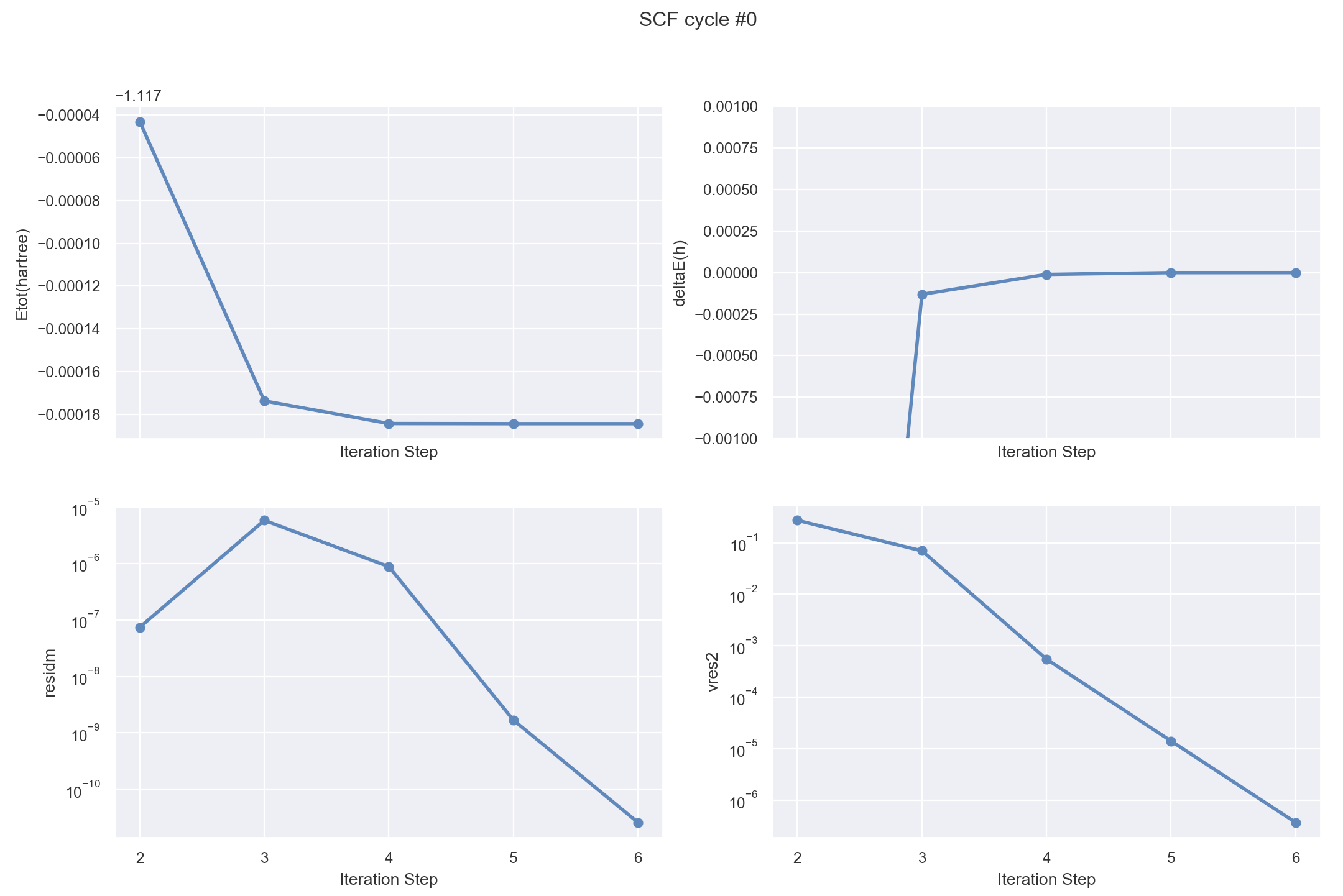
6 SCF cycles were needed:
     iter   Etot(hartree)      deltaE(h)  residm     vres2
 ETOT  1  -1.1093804698962    -1.109E+00 6.384E-04 1.736E+01
 ETOT  2  -1.1170431098364    -7.663E-03 7.449E-08 2.737E-01
 ETOT  3  -1.1171736936408    -1.306E-04 5.867E-06 6.992E-02
 ETOT  4  -1.1171842773283    -1.058E-05 8.862E-07 5.492E-04
 ETOT  5  -1.1171843458762    -6.855E-08 1.683E-09 1.404E-05
 ETOT  6  -1.1171843463443    -4.681E-10 2.580E-11 3.672E-07

 At SCF step    6, etot is converged :
  for the second time, diff in etot=  4.681E-10 < toldfe=  1.000E-06
Note that the number of steps that were allowed, nstep = 10, is larger than the number of steps effectively needed to reach the stopping criterion. As a rule, you should always check that the number of steps that you allowed was sufficient to reach the target tolerance. You might now play a bit with nstep, as e.g. set it to 5, to see how abinit reacts.
Side note: in most of the tutorial examples, nstep will be enough to reach the target tolerance, defined by one of the tolXXX input variables. However, this is not always the case (e.g. the test case 1 of the tutorial DFPT1 because of some portability problems, that could only be solved by stopping the SCF cycles before the required tolerance.
Q2. Is the energy likely more converged than toldfe?
The information is contained in the same piece of the output file. Yes, the energy is more converged than toldfe, since the stopping criterion asked for the difference between successive evaluations of the energy to be smaller than toldfe twice in a row, while the evolution of the energy is nice, and always decreasing by smaller and smaller amounts.
Q3. What is the value of the force on each atom, in Ha/Bohr?
These values are:
 cartesian_forces: # hartree/bohr
 - [ -2.69021104E-02,  -0.00000000E+00,  -0.00000000E+00, ]
 - [  2.69021104E-02,  -0.00000000E+00,  -0.00000000E+00, ]
 force_length_stats: {min:   2.69021104E-02, max:   2.69021104E-02, mean:   2.69021104E-02, }
On the first atom (located at -0.7 0 0 in cartesian coordinates, in Bohr), the force vector is pointing in the \(-x\) direction, and in the \(+x\) direction for the second atom located at +0.7 0 0 . The H\(_2\) molecule would like to expand…
Q4. What is the difference of eigenenergies between the two electronic states?
The eigenvalues (in Hartree) are mentioned at the lines
Eigenvalues (hartree) for nkpt=   1  k points:
kpt#   1, nband=  2, wtk=  1.00000, kpt=  0.0000  0.0000  0.0000 (reduced coord)
-0.36942   -0.01446
As mentioned in the abinit help file the absolute value of eigenenergies is not meaningful. Only differences of eigenenergies, as well as differences with the potential. The difference is 0.35496 Hartree, that is 9.6588 eV . Moreover, remember that Kohn-Sham eigenenergies are formally not connected to experimental excitation energies! (Well, more is to be said later about this in the GW tutorials).
Q5. Can you set prtvol to 2 in the input file, run again abinit, and find where is located the maximum of the electronic density, and how much is it, in electrons/Bohr^3 ?
The maximum electronic density in electron per Bohr cube is reached at the mid-point between the two H atoms:
Total charge density [el/Bohr^3]
      Maximum=    2.7281E-01  at reduced coord.    0.0000    0.0000    0.0000
Tip
If AbiPy is installed on your machine, you can use the abiopen.py script
with the --expose option to visualize the SCF cycle from the main output file:
abiopen.py tbase1_1.abo --expose --seaborn
For further info, please consult this jupyter notebook that reformulates the present tutorial using AbiPy.
Computation of the interatomic distance (method 1)
Starting from now, every time a new input variable is mentioned, you should read the corresponding descriptive section in the abinit help file.
We will now complete the description of the meaning of each term: there are still a few indications that you should be aware of, even if you will not use them in the tutorial. These might appear in the description of some input variables. For this, you should read the section 3.3 of the abinit help file.
There are three methodologies to compute the optimal distance between the two Hydrogen atoms. One could:
- compute the total energy for different values of the interatomic distance, make a fit through the different points, and determine the minimum of the fitting function;
- compute the forces for different values of the interatomic distance, make a fit through the different values, and determine the zero of the fitting function;
- use an automatic algorithm for minimizing the energy (or finding the zero of forces).
We will begin with the computation of energy and forces for different values of the interatomic distance. This exercise will allow you to learn how to use multiple datasets.
The interatomic distance in the tbase1_1.abi file was 1.4 Bohr. Suppose you decide to examine the interatomic distances from 1.0 Bohr to 2.0 Bohr, by steps of 0.05 Bohr. That is, 21 calculations. If you are a UNIX guru, it will be easy for you to write a script that will drive these 21 calculations, changing automatically the variable xcart in the input file, and then gather all the data, in a convenient form to be plotted.
Well, are you a UNIX guru? If not, there is an easier path, all within abinit! This is the multi-dataset mode. Detailed explanations about it can be found in sections 3.4, 3.5, 3.6 and 3.7 of the abinit help file.
Now, can you write an input file that will do the computation described above (interatomic distances from 1.0 Bohr to 2.0 Bohr, by steps of 0.05 Bohr)? You might start from tbase1_1.abi. Try to define a series, and to use the getwfk input variable (the latter will make the computation much faster).
You should likely have a look at the section that describes the irdwfk and getwfk input variables: in particular, look at the meaning of getwfk -1 Also, define explicitly the number of states (or supercell “bands”) to be one, using the input variable nband.
The input file $ABI_TESTS/tutorial/Input/tbase1_2.abi is an example of file that will do the job,
# H2 molecule in a big box
#
# This file to compute the total energy and forces as a function
# of the interatomic distance

#Define the different datasets
ndtset 21               # 21 datasets
xcart:  -0.5   0.0 0.0  # The starting values of the
         0.5   0.0 0.0  # atomic coordinates
xcart+  -0.025 0.0 0.0  # The increment of xcart from one dataset to the other
         0.025 0.0 0.0  #
getwfk  -1              # Will use the converged wavefunction from the
                        # previous dataset to start the new dataset computation
nband    1              # Only one band is occupied. In order to get the energy,
                        # there is no need to compute more than one band.

#-------------------------------------------------------------------------------
#The rest of this file is similar to the tbase1_1.in file, except
#that xcart has been moved above ...

#Definition of the unit cell
acell 10 10 10    # The keyword "acell" refers to the
                  # lengths of the primitive vectors (in Bohr)
#rprim 1 0 0  0 1 0  0 0 1 # This line, defining orthogonal primitive vectors,
                           # is commented, because it is precisely the default value of rprim

#Definition of the atom types and pseudopotentials
ntypat 1          # There is only one type of atom
znucl 1           # The keyword "znucl" refers to the atomic number of the possible type(s) of atom.
                  # Here, the only type is Hydrogen. The pseudopotential(s)
                  # mentioned after the keyword "pseudos" should correspond to this type of atom.
pp_dirpath "$ABI_PSPDIR"                 # This is the path to the directory were pseudopotentials for tests are stored
pseudos "Psdj_nc_sr_04_pw_std_psp8/H.psp8"  # Name and location of the pseudopotential
                  # This pseudopotential comes from the pseudodojo site http://www.pseudo-dojo.org/  (NC SR LDA standard),
                  # and was generated using the LDA exchange-correlation functional (PW=Perdew-Wang, ixc=-1012).
                  # By default, abinit uses the same exchange-correlation functional than the one of the input pseudopotential(s)

#Definition of the atoms
natom 2           # There are two atoms
typat  1 1        # They both are of type 1, that is, Hydrogen

#Numerical parameters of the calculation : planewave basis set and k point grid
ecut 10.0         # Maximal plane-wave kinetic energy cut-off, in Hartree
kptopt 0          # Enter the k points manually
nkpt 1            # Only one k point is needed for isolated system,
                  # taken by default to be 0.0 0.0 0.0

#Parameters for the SCF procedure
nstep 10          # Maximal number of SCF cycles
toldfe 1.0d-6     # Will stop when, twice in a row, the difference
                  # between two consecutive evaluations of total energy
                  # differ by less than toldfe (in Hartree)
                  # This value is way too large for most realistic studies of materials
diemac 2.0        # Although this is not mandatory, it is worth to
                  # precondition the SCF cycle. The model dielectric
                  # function used as the standard preconditioner
                  # is described in the "dielng" input variable section.
                  # Here, we follow the prescriptions for molecules
                  # in a big box

##############################################################
# This section is used only for regression testing of ABINIT #
##############################################################
#%%<BEGIN TEST_INFO>
#%% [setup]
#%% executable = abinit
#%% [files]
#%% files_to_test =
#%%   tbase1_2.abo, tolnlines=  0, tolabs=  0.000e+00, tolrel=  0.000e+00
#%% [paral_info]
#%% max_nprocs = 1
#%% [extra_info]
#%% authors = X. Gonze
#%% keywords =
#%% description =
#%%  H2 molecule in a big box
#%%  This file to compute the total energy and forces as a function
#%%  of the interatomic distance
#%%<END TEST_INFO>
while $ABI_TESTS/tutorial/Refs/tbase1_2.abo is the reference output file.
.Version 10.5.8.2 of ABINIT, released Oct 2025.
.(MPI version, prepared for a x86_64_linux_gnu13.2 computer)
.Copyright (C) 1998-2026 ABINIT group .
ABINIT comes with ABSOLUTELY NO WARRANTY.
It is free software, and you are welcome to redistribute it
under certain conditions (GNU General Public License,
see ~abinit/COPYING or http://www.gnu.org/copyleft/gpl.txt).
ABINIT is a project of the Universite Catholique de Louvain,
Corning Inc. and other collaborators, see ~abinit/doc/developers/contributors.txt .
Please read https://docs.abinit.org/theory/acknowledgments for suggested
acknowledgments of the ABINIT effort.
For more information, see https://www.abinit.org .
.Starting date : Sat 20 Dec 2025.
- ( at 17h05 )
- input file -> /home/buildbot/ABINIT3/eos_gnu_13.2_mpich/trunk__codata2022/tests/TestBot_MPI1/tutorial_tbase1_2/tbase1_2.abi
- output file -> tbase1_2.abo
- root for input files -> tbase1_2i
- root for output files -> tbase1_2o
DATASET 1 : space group P4/m m m (#123); Bravais tP (primitive tetrag.)
================================================================================
Values of the parameters that define the memory need for DATASET 1.
intxc = 0 ionmov = 0 iscf = 7 lmnmax = 3
lnmax = 3 mgfft = 30 mpssoang = 2 mqgrid = 3001
natom = 2 nloc_mem = 1 nspden = 1 nspinor = 1
nsppol = 1 nsym = 16 n1xccc = 0 ntypat = 1
occopt = 1 xclevel = 1
- mband = 1 mffmem = 1 mkmem = 1
mpw = 752 nfft = 27000 nkpt = 1
================================================================================
P This job should need less than 8.700 Mbytes of memory.
Rough estimation (10% accuracy) of disk space for files :
_ WF disk file : 0.013 Mbytes ; DEN or POT disk file : 0.208 Mbytes.
================================================================================
DATASET 2 : space group P4/m m m (#123); Bravais tP (primitive tetrag.)
================================================================================
Values of the parameters that define the memory need for DATASET 2.
intxc = 0 ionmov = 0 iscf = 7 lmnmax = 3
lnmax = 3 mgfft = 30 mpssoang = 2 mqgrid = 3001
natom = 2 nloc_mem = 1 nspden = 1 nspinor = 1
nsppol = 1 nsym = 16 n1xccc = 0 ntypat = 1
occopt = 1 xclevel = 1
- mband = 1 mffmem = 1 mkmem = 1
mpw = 752 nfft = 27000 nkpt = 1
================================================================================
P This job should need less than 8.700 Mbytes of memory.
Rough estimation (10% accuracy) of disk space for files :
_ WF disk file : 0.013 Mbytes ; DEN or POT disk file : 0.208 Mbytes.
================================================================================
DATASET 3 : space group P4/m m m (#123); Bravais tP (primitive tetrag.)
================================================================================
Values of the parameters that define the memory need for DATASET 3.
intxc = 0 ionmov = 0 iscf = 7 lmnmax = 3
lnmax = 3 mgfft = 30 mpssoang = 2 mqgrid = 3001
natom = 2 nloc_mem = 1 nspden = 1 nspinor = 1
nsppol = 1 nsym = 16 n1xccc = 0 ntypat = 1
occopt = 1 xclevel = 1
- mband = 1 mffmem = 1 mkmem = 1
mpw = 752 nfft = 27000 nkpt = 1
================================================================================
P This job should need less than 8.700 Mbytes of memory.
Rough estimation (10% accuracy) of disk space for files :
_ WF disk file : 0.013 Mbytes ; DEN or POT disk file : 0.208 Mbytes.
================================================================================
DATASET 4 : space group P4/m m m (#123); Bravais tP (primitive tetrag.)
================================================================================
Values of the parameters that define the memory need for DATASET 4.
intxc = 0 ionmov = 0 iscf = 7 lmnmax = 3
lnmax = 3 mgfft = 30 mpssoang = 2 mqgrid = 3001
natom = 2 nloc_mem = 1 nspden = 1 nspinor = 1
nsppol = 1 nsym = 16 n1xccc = 0 ntypat = 1
occopt = 1 xclevel = 1
- mband = 1 mffmem = 1 mkmem = 1
mpw = 752 nfft = 27000 nkpt = 1
================================================================================
P This job should need less than 8.700 Mbytes of memory.
Rough estimation (10% accuracy) of disk space for files :
_ WF disk file : 0.013 Mbytes ; DEN or POT disk file : 0.208 Mbytes.
================================================================================
DATASET 5 : space group P4/m m m (#123); Bravais tP (primitive tetrag.)
================================================================================
Values of the parameters that define the memory need for DATASET 5.
intxc = 0 ionmov = 0 iscf = 7 lmnmax = 3
lnmax = 3 mgfft = 30 mpssoang = 2 mqgrid = 3001
natom = 2 nloc_mem = 1 nspden = 1 nspinor = 1
nsppol = 1 nsym = 16 n1xccc = 0 ntypat = 1
occopt = 1 xclevel = 1
- mband = 1 mffmem = 1 mkmem = 1
mpw = 752 nfft = 27000 nkpt = 1
================================================================================
P This job should need less than 8.700 Mbytes of memory.
Rough estimation (10% accuracy) of disk space for files :
_ WF disk file : 0.013 Mbytes ; DEN or POT disk file : 0.208 Mbytes.
================================================================================
DATASET 6 : space group P4/m m m (#123); Bravais tP (primitive tetrag.)
================================================================================
Values of the parameters that define the memory need for DATASET 6.
intxc = 0 ionmov = 0 iscf = 7 lmnmax = 3
lnmax = 3 mgfft = 30 mpssoang = 2 mqgrid = 3001
natom = 2 nloc_mem = 1 nspden = 1 nspinor = 1
nsppol = 1 nsym = 16 n1xccc = 0 ntypat = 1
occopt = 1 xclevel = 1
- mband = 1 mffmem = 1 mkmem = 1
mpw = 752 nfft = 27000 nkpt = 1
================================================================================
P This job should need less than 8.700 Mbytes of memory.
Rough estimation (10% accuracy) of disk space for files :
_ WF disk file : 0.013 Mbytes ; DEN or POT disk file : 0.208 Mbytes.
================================================================================
DATASET 7 : space group P4/m m m (#123); Bravais tP (primitive tetrag.)
================================================================================
Values of the parameters that define the memory need for DATASET 7.
intxc = 0 ionmov = 0 iscf = 7 lmnmax = 3
lnmax = 3 mgfft = 30 mpssoang = 2 mqgrid = 3001
natom = 2 nloc_mem = 1 nspden = 1 nspinor = 1
nsppol = 1 nsym = 16 n1xccc = 0 ntypat = 1
occopt = 1 xclevel = 1
- mband = 1 mffmem = 1 mkmem = 1
mpw = 752 nfft = 27000 nkpt = 1
================================================================================
P This job should need less than 8.700 Mbytes of memory.
Rough estimation (10% accuracy) of disk space for files :
_ WF disk file : 0.013 Mbytes ; DEN or POT disk file : 0.208 Mbytes.
================================================================================
DATASET 8 : space group P4/m m m (#123); Bravais tP (primitive tetrag.)
================================================================================
Values of the parameters that define the memory need for DATASET 8.
intxc = 0 ionmov = 0 iscf = 7 lmnmax = 3
lnmax = 3 mgfft = 30 mpssoang = 2 mqgrid = 3001
natom = 2 nloc_mem = 1 nspden = 1 nspinor = 1
nsppol = 1 nsym = 16 n1xccc = 0 ntypat = 1
occopt = 1 xclevel = 1
- mband = 1 mffmem = 1 mkmem = 1
mpw = 752 nfft = 27000 nkpt = 1
================================================================================
P This job should need less than 8.700 Mbytes of memory.
Rough estimation (10% accuracy) of disk space for files :
_ WF disk file : 0.013 Mbytes ; DEN or POT disk file : 0.208 Mbytes.
================================================================================
DATASET 9 : space group P4/m m m (#123); Bravais tP (primitive tetrag.)
================================================================================
Values of the parameters that define the memory need for DATASET 9.
intxc = 0 ionmov = 0 iscf = 7 lmnmax = 3
lnmax = 3 mgfft = 30 mpssoang = 2 mqgrid = 3001
natom = 2 nloc_mem = 1 nspden = 1 nspinor = 1
nsppol = 1 nsym = 16 n1xccc = 0 ntypat = 1
occopt = 1 xclevel = 1
- mband = 1 mffmem = 1 mkmem = 1
mpw = 752 nfft = 27000 nkpt = 1
================================================================================
P This job should need less than 8.700 Mbytes of memory.
Rough estimation (10% accuracy) of disk space for files :
_ WF disk file : 0.013 Mbytes ; DEN or POT disk file : 0.208 Mbytes.
================================================================================
DATASET 10 : space group P4/m m m (#123); Bravais tP (primitive tetrag.)
================================================================================
Values of the parameters that define the memory need for DATASET 10.
intxc = 0 ionmov = 0 iscf = 7 lmnmax = 3
lnmax = 3 mgfft = 30 mpssoang = 2 mqgrid = 3001
natom = 2 nloc_mem = 1 nspden = 1 nspinor = 1
nsppol = 1 nsym = 16 n1xccc = 0 ntypat = 1
occopt = 1 xclevel = 1
- mband = 1 mffmem = 1 mkmem = 1
mpw = 752 nfft = 27000 nkpt = 1
================================================================================
P This job should need less than 8.700 Mbytes of memory.
Rough estimation (10% accuracy) of disk space for files :
_ WF disk file : 0.013 Mbytes ; DEN or POT disk file : 0.208 Mbytes.
================================================================================
DATASET 11 : space group P4/m m m (#123); Bravais tP (primitive tetrag.)
================================================================================
Values of the parameters that define the memory need for DATASET 11.
intxc = 0 ionmov = 0 iscf = 7 lmnmax = 3
lnmax = 3 mgfft = 30 mpssoang = 2 mqgrid = 3001
natom = 2 nloc_mem = 1 nspden = 1 nspinor = 1
nsppol = 1 nsym = 16 n1xccc = 0 ntypat = 1
occopt = 1 xclevel = 1
- mband = 1 mffmem = 1 mkmem = 1
mpw = 752 nfft = 27000 nkpt = 1
================================================================================
P This job should need less than 8.700 Mbytes of memory.
Rough estimation (10% accuracy) of disk space for files :
_ WF disk file : 0.013 Mbytes ; DEN or POT disk file : 0.208 Mbytes.
================================================================================
DATASET 12 : space group P4/m m m (#123); Bravais tP (primitive tetrag.)
================================================================================
Values of the parameters that define the memory need for DATASET 12.
intxc = 0 ionmov = 0 iscf = 7 lmnmax = 3
lnmax = 3 mgfft = 30 mpssoang = 2 mqgrid = 3001
natom = 2 nloc_mem = 1 nspden = 1 nspinor = 1
nsppol = 1 nsym = 16 n1xccc = 0 ntypat = 1
occopt = 1 xclevel = 1
- mband = 1 mffmem = 1 mkmem = 1
mpw = 752 nfft = 27000 nkpt = 1
================================================================================
P This job should need less than 8.700 Mbytes of memory.
Rough estimation (10% accuracy) of disk space for files :
_ WF disk file : 0.013 Mbytes ; DEN or POT disk file : 0.208 Mbytes.
================================================================================
DATASET 13 : space group P4/m m m (#123); Bravais tP (primitive tetrag.)
================================================================================
Values of the parameters that define the memory need for DATASET 13.
intxc = 0 ionmov = 0 iscf = 7 lmnmax = 3
lnmax = 3 mgfft = 30 mpssoang = 2 mqgrid = 3001
natom = 2 nloc_mem = 1 nspden = 1 nspinor = 1
nsppol = 1 nsym = 16 n1xccc = 0 ntypat = 1
occopt = 1 xclevel = 1
- mband = 1 mffmem = 1 mkmem = 1
mpw = 752 nfft = 27000 nkpt = 1
================================================================================
P This job should need less than 8.700 Mbytes of memory.
Rough estimation (10% accuracy) of disk space for files :
_ WF disk file : 0.013 Mbytes ; DEN or POT disk file : 0.208 Mbytes.
================================================================================
DATASET 14 : space group P4/m m m (#123); Bravais tP (primitive tetrag.)
================================================================================
Values of the parameters that define the memory need for DATASET 14.
intxc = 0 ionmov = 0 iscf = 7 lmnmax = 3
lnmax = 3 mgfft = 30 mpssoang = 2 mqgrid = 3001
natom = 2 nloc_mem = 1 nspden = 1 nspinor = 1
nsppol = 1 nsym = 16 n1xccc = 0 ntypat = 1
occopt = 1 xclevel = 1
- mband = 1 mffmem = 1 mkmem = 1
mpw = 752 nfft = 27000 nkpt = 1
================================================================================
P This job should need less than 8.700 Mbytes of memory.
Rough estimation (10% accuracy) of disk space for files :
_ WF disk file : 0.013 Mbytes ; DEN or POT disk file : 0.208 Mbytes.
================================================================================
DATASET 15 : space group P4/m m m (#123); Bravais tP (primitive tetrag.)
================================================================================
Values of the parameters that define the memory need for DATASET 15.
intxc = 0 ionmov = 0 iscf = 7 lmnmax = 3
lnmax = 3 mgfft = 30 mpssoang = 2 mqgrid = 3001
natom = 2 nloc_mem = 1 nspden = 1 nspinor = 1
nsppol = 1 nsym = 16 n1xccc = 0 ntypat = 1
occopt = 1 xclevel = 1
- mband = 1 mffmem = 1 mkmem = 1
mpw = 752 nfft = 27000 nkpt = 1
================================================================================
P This job should need less than 8.700 Mbytes of memory.
Rough estimation (10% accuracy) of disk space for files :
_ WF disk file : 0.013 Mbytes ; DEN or POT disk file : 0.208 Mbytes.
================================================================================
DATASET 16 : space group P4/m m m (#123); Bravais tP (primitive tetrag.)
================================================================================
Values of the parameters that define the memory need for DATASET 16.
intxc = 0 ionmov = 0 iscf = 7 lmnmax = 3
lnmax = 3 mgfft = 30 mpssoang = 2 mqgrid = 3001
natom = 2 nloc_mem = 1 nspden = 1 nspinor = 1
nsppol = 1 nsym = 16 n1xccc = 0 ntypat = 1
occopt = 1 xclevel = 1
- mband = 1 mffmem = 1 mkmem = 1
mpw = 752 nfft = 27000 nkpt = 1
================================================================================
P This job should need less than 8.700 Mbytes of memory.
Rough estimation (10% accuracy) of disk space for files :
_ WF disk file : 0.013 Mbytes ; DEN or POT disk file : 0.208 Mbytes.
================================================================================
DATASET 17 : space group P4/m m m (#123); Bravais tP (primitive tetrag.)
================================================================================
Values of the parameters that define the memory need for DATASET 17.
intxc = 0 ionmov = 0 iscf = 7 lmnmax = 3
lnmax = 3 mgfft = 30 mpssoang = 2 mqgrid = 3001
natom = 2 nloc_mem = 1 nspden = 1 nspinor = 1
nsppol = 1 nsym = 16 n1xccc = 0 ntypat = 1
occopt = 1 xclevel = 1
- mband = 1 mffmem = 1 mkmem = 1
mpw = 752 nfft = 27000 nkpt = 1
================================================================================
P This job should need less than 8.700 Mbytes of memory.
Rough estimation (10% accuracy) of disk space for files :
_ WF disk file : 0.013 Mbytes ; DEN or POT disk file : 0.208 Mbytes.
================================================================================
DATASET 18 : space group P4/m m m (#123); Bravais tP (primitive tetrag.)
================================================================================
Values of the parameters that define the memory need for DATASET 18.
intxc = 0 ionmov = 0 iscf = 7 lmnmax = 3
lnmax = 3 mgfft = 30 mpssoang = 2 mqgrid = 3001
natom = 2 nloc_mem = 1 nspden = 1 nspinor = 1
nsppol = 1 nsym = 16 n1xccc = 0 ntypat = 1
occopt = 1 xclevel = 1
- mband = 1 mffmem = 1 mkmem = 1
mpw = 752 nfft = 27000 nkpt = 1
================================================================================
P This job should need less than 8.700 Mbytes of memory.
Rough estimation (10% accuracy) of disk space for files :
_ WF disk file : 0.013 Mbytes ; DEN or POT disk file : 0.208 Mbytes.
================================================================================
DATASET 19 : space group P4/m m m (#123); Bravais tP (primitive tetrag.)
================================================================================
Values of the parameters that define the memory need for DATASET 19.
intxc = 0 ionmov = 0 iscf = 7 lmnmax = 3
lnmax = 3 mgfft = 30 mpssoang = 2 mqgrid = 3001
natom = 2 nloc_mem = 1 nspden = 1 nspinor = 1
nsppol = 1 nsym = 16 n1xccc = 0 ntypat = 1
occopt = 1 xclevel = 1
- mband = 1 mffmem = 1 mkmem = 1
mpw = 752 nfft = 27000 nkpt = 1
================================================================================
P This job should need less than 8.700 Mbytes of memory.
Rough estimation (10% accuracy) of disk space for files :
_ WF disk file : 0.013 Mbytes ; DEN or POT disk file : 0.208 Mbytes.
================================================================================
DATASET 20 : space group P4/m m m (#123); Bravais tP (primitive tetrag.)
================================================================================
Values of the parameters that define the memory need for DATASET 20.
intxc = 0 ionmov = 0 iscf = 7 lmnmax = 3
lnmax = 3 mgfft = 30 mpssoang = 2 mqgrid = 3001
natom = 2 nloc_mem = 1 nspden = 1 nspinor = 1
nsppol = 1 nsym = 16 n1xccc = 0 ntypat = 1
occopt = 1 xclevel = 1
- mband = 1 mffmem = 1 mkmem = 1
mpw = 752 nfft = 27000 nkpt = 1
================================================================================
P This job should need less than 8.700 Mbytes of memory.
Rough estimation (10% accuracy) of disk space for files :
_ WF disk file : 0.013 Mbytes ; DEN or POT disk file : 0.208 Mbytes.
================================================================================
DATASET 21 : space group P4/m m m (#123); Bravais tP (primitive tetrag.)
================================================================================
Values of the parameters that define the memory need for DATASET 21.
intxc = 0 ionmov = 0 iscf = 7 lmnmax = 3
lnmax = 3 mgfft = 30 mpssoang = 2 mqgrid = 3001
natom = 2 nloc_mem = 1 nspden = 1 nspinor = 1
nsppol = 1 nsym = 16 n1xccc = 0 ntypat = 1
occopt = 1 xclevel = 1
- mband = 1 mffmem = 1 mkmem = 1
mpw = 752 nfft = 27000 nkpt = 1
================================================================================
P This job should need less than 8.700 Mbytes of memory.
Rough estimation (10% accuracy) of disk space for files :
_ WF disk file : 0.013 Mbytes ; DEN or POT disk file : 0.208 Mbytes.
================================================================================
--------------------------------------------------------------------------------
------------- Echo of variables that govern the present computation ------------
--------------------------------------------------------------------------------
-
- outvars: echo of selected default values
- iomode0 = 0 , fftalg0 =512 , wfoptalg0 = 0
-
- outvars: echo of global parameters not present in the input file
- max_nthreads = 0
-
-outvars: echo values of preprocessed input variables --------
acell 1.0000000000E+01 1.0000000000E+01 1.0000000000E+01 Bohr
amu 1.00794000E+00
diemac 2.00000000E+00
ecut 1.00000000E+01 Hartree
- fftalg 512
getwfk -1
istwfk 2
ixc -1012
jdtset 1 2 3 4 5 6 7 8 9 10
11 12 13 14 15 16 17 18 19 20
21
kptopt 0
P mkmem 1
natom 2
nband 1
ndtset 21
ngfft 30 30 30
nkpt 1
nstep 10
nsym 16
ntypat 1
occ 2.000000
spgroup 123
symrel 1 0 0 0 1 0 0 0 1 -1 0 0 0 -1 0 0 0 -1
-1 0 0 0 1 0 0 0 -1 1 0 0 0 -1 0 0 0 1
-1 0 0 0 -1 0 0 0 1 1 0 0 0 1 0 0 0 -1
1 0 0 0 -1 0 0 0 -1 -1 0 0 0 1 0 0 0 1
1 0 0 0 0 1 0 1 0 -1 0 0 0 0 -1 0 -1 0
-1 0 0 0 0 1 0 -1 0 1 0 0 0 0 -1 0 1 0
-1 0 0 0 0 -1 0 1 0 1 0 0 0 0 1 0 -1 0
1 0 0 0 0 -1 0 -1 0 -1 0 0 0 0 1 0 1 0
toldfe 1.00000000E-06 Hartree
typat 1 1
xangst1 -2.6458860527E-01 0.0000000000E+00 0.0000000000E+00
2.6458860527E-01 0.0000000000E+00 0.0000000000E+00
xangst2 -2.7781803554E-01 0.0000000000E+00 0.0000000000E+00
2.7781803554E-01 0.0000000000E+00 0.0000000000E+00
xangst3 -2.9104746580E-01 0.0000000000E+00 0.0000000000E+00
2.9104746580E-01 0.0000000000E+00 0.0000000000E+00
xangst4 -3.0427689606E-01 0.0000000000E+00 0.0000000000E+00
3.0427689606E-01 0.0000000000E+00 0.0000000000E+00
xangst5 -3.1750632633E-01 0.0000000000E+00 0.0000000000E+00
3.1750632633E-01 0.0000000000E+00 0.0000000000E+00
xangst6 -3.3073575659E-01 0.0000000000E+00 0.0000000000E+00
3.3073575659E-01 0.0000000000E+00 0.0000000000E+00
xangst7 -3.4396518685E-01 0.0000000000E+00 0.0000000000E+00
3.4396518685E-01 0.0000000000E+00 0.0000000000E+00
xangst8 -3.5719461712E-01 0.0000000000E+00 0.0000000000E+00
3.5719461712E-01 0.0000000000E+00 0.0000000000E+00
xangst9 -3.7042404738E-01 0.0000000000E+00 0.0000000000E+00
3.7042404738E-01 0.0000000000E+00 0.0000000000E+00
xangst10 -3.8365347764E-01 0.0000000000E+00 0.0000000000E+00
3.8365347764E-01 0.0000000000E+00 0.0000000000E+00
xangst11 -3.9688290791E-01 0.0000000000E+00 0.0000000000E+00
3.9688290791E-01 0.0000000000E+00 0.0000000000E+00
xangst12 -4.1011233817E-01 0.0000000000E+00 0.0000000000E+00
4.1011233817E-01 0.0000000000E+00 0.0000000000E+00
xangst13 -4.2334176844E-01 0.0000000000E+00 0.0000000000E+00
4.2334176844E-01 0.0000000000E+00 0.0000000000E+00
xangst14 -4.3657119870E-01 0.0000000000E+00 0.0000000000E+00
4.3657119870E-01 0.0000000000E+00 0.0000000000E+00
xangst15 -4.4980062896E-01 0.0000000000E+00 0.0000000000E+00
4.4980062896E-01 0.0000000000E+00 0.0000000000E+00
xangst16 -4.6303005923E-01 0.0000000000E+00 0.0000000000E+00
4.6303005923E-01 0.0000000000E+00 0.0000000000E+00
xangst17 -4.7625948949E-01 0.0000000000E+00 0.0000000000E+00
4.7625948949E-01 0.0000000000E+00 0.0000000000E+00
xangst18 -4.8948891975E-01 0.0000000000E+00 0.0000000000E+00
4.8948891975E-01 0.0000000000E+00 0.0000000000E+00
xangst19 -5.0271835002E-01 0.0000000000E+00 0.0000000000E+00
5.0271835002E-01 0.0000000000E+00 0.0000000000E+00
xangst20 -5.1594778028E-01 0.0000000000E+00 0.0000000000E+00
5.1594778028E-01 0.0000000000E+00 0.0000000000E+00
xangst21 -5.2917721054E-01 0.0000000000E+00 0.0000000000E+00
5.2917721054E-01 0.0000000000E+00 0.0000000000E+00
xcart1 -5.0000000000E-01 0.0000000000E+00 0.0000000000E+00
5.0000000000E-01 0.0000000000E+00 0.0000000000E+00
xcart2 -5.2500000000E-01 0.0000000000E+00 0.0000000000E+00
5.2500000000E-01 0.0000000000E+00 0.0000000000E+00
xcart3 -5.5000000000E-01 0.0000000000E+00 0.0000000000E+00
5.5000000000E-01 0.0000000000E+00 0.0000000000E+00
xcart4 -5.7500000000E-01 0.0000000000E+00 0.0000000000E+00
5.7500000000E-01 0.0000000000E+00 0.0000000000E+00
xcart5 -6.0000000000E-01 0.0000000000E+00 0.0000000000E+00
6.0000000000E-01 0.0000000000E+00 0.0000000000E+00
xcart6 -6.2500000000E-01 0.0000000000E+00 0.0000000000E+00
6.2500000000E-01 0.0000000000E+00 0.0000000000E+00
xcart7 -6.5000000000E-01 0.0000000000E+00 0.0000000000E+00
6.5000000000E-01 0.0000000000E+00 0.0000000000E+00
xcart8 -6.7500000000E-01 0.0000000000E+00 0.0000000000E+00
6.7500000000E-01 0.0000000000E+00 0.0000000000E+00
xcart9 -7.0000000000E-01 0.0000000000E+00 0.0000000000E+00
7.0000000000E-01 0.0000000000E+00 0.0000000000E+00
xcart10 -7.2500000000E-01 0.0000000000E+00 0.0000000000E+00
7.2500000000E-01 0.0000000000E+00 0.0000000000E+00
xcart11 -7.5000000000E-01 0.0000000000E+00 0.0000000000E+00
7.5000000000E-01 0.0000000000E+00 0.0000000000E+00
xcart12 -7.7500000000E-01 0.0000000000E+00 0.0000000000E+00
7.7500000000E-01 0.0000000000E+00 0.0000000000E+00
xcart13 -8.0000000000E-01 0.0000000000E+00 0.0000000000E+00
8.0000000000E-01 0.0000000000E+00 0.0000000000E+00
xcart14 -8.2500000000E-01 0.0000000000E+00 0.0000000000E+00
8.2500000000E-01 0.0000000000E+00 0.0000000000E+00
xcart15 -8.5000000000E-01 0.0000000000E+00 0.0000000000E+00
8.5000000000E-01 0.0000000000E+00 0.0000000000E+00
xcart16 -8.7500000000E-01 0.0000000000E+00 0.0000000000E+00
8.7500000000E-01 0.0000000000E+00 0.0000000000E+00
xcart17 -9.0000000000E-01 0.0000000000E+00 0.0000000000E+00
9.0000000000E-01 0.0000000000E+00 0.0000000000E+00
xcart18 -9.2500000000E-01 0.0000000000E+00 0.0000000000E+00
9.2500000000E-01 0.0000000000E+00 0.0000000000E+00
xcart19 -9.5000000000E-01 0.0000000000E+00 0.0000000000E+00
9.5000000000E-01 0.0000000000E+00 0.0000000000E+00
xcart20 -9.7500000000E-01 0.0000000000E+00 0.0000000000E+00
9.7500000000E-01 0.0000000000E+00 0.0000000000E+00
xcart21 -1.0000000000E+00 0.0000000000E+00 0.0000000000E+00
1.0000000000E+00 0.0000000000E+00 0.0000000000E+00
xred1 -5.0000000000E-02 0.0000000000E+00 0.0000000000E+00
5.0000000000E-02 0.0000000000E+00 0.0000000000E+00
xred2 -5.2500000000E-02 0.0000000000E+00 0.0000000000E+00
5.2500000000E-02 0.0000000000E+00 0.0000000000E+00
xred3 -5.5000000000E-02 0.0000000000E+00 0.0000000000E+00
5.5000000000E-02 0.0000000000E+00 0.0000000000E+00
xred4 -5.7500000000E-02 0.0000000000E+00 0.0000000000E+00
5.7500000000E-02 0.0000000000E+00 0.0000000000E+00
xred5 -6.0000000000E-02 0.0000000000E+00 0.0000000000E+00
6.0000000000E-02 0.0000000000E+00 0.0000000000E+00
xred6 -6.2500000000E-02 0.0000000000E+00 0.0000000000E+00
6.2500000000E-02 0.0000000000E+00 0.0000000000E+00
xred7 -6.5000000000E-02 0.0000000000E+00 0.0000000000E+00
6.5000000000E-02 0.0000000000E+00 0.0000000000E+00
xred8 -6.7500000000E-02 0.0000000000E+00 0.0000000000E+00
6.7500000000E-02 0.0000000000E+00 0.0000000000E+00
xred9 -7.0000000000E-02 0.0000000000E+00 0.0000000000E+00
7.0000000000E-02 0.0000000000E+00 0.0000000000E+00
xred10 -7.2500000000E-02 0.0000000000E+00 0.0000000000E+00
7.2500000000E-02 0.0000000000E+00 0.0000000000E+00
xred11 -7.5000000000E-02 0.0000000000E+00 0.0000000000E+00
7.5000000000E-02 0.0000000000E+00 0.0000000000E+00
xred12 -7.7500000000E-02 0.0000000000E+00 0.0000000000E+00
7.7500000000E-02 0.0000000000E+00 0.0000000000E+00
xred13 -8.0000000000E-02 0.0000000000E+00 0.0000000000E+00
8.0000000000E-02 0.0000000000E+00 0.0000000000E+00
xred14 -8.2500000000E-02 0.0000000000E+00 0.0000000000E+00
8.2500000000E-02 0.0000000000E+00 0.0000000000E+00
xred15 -8.5000000000E-02 0.0000000000E+00 0.0000000000E+00
8.5000000000E-02 0.0000000000E+00 0.0000000000E+00
xred16 -8.7500000000E-02 0.0000000000E+00 0.0000000000E+00
8.7500000000E-02 0.0000000000E+00 0.0000000000E+00
xred17 -9.0000000000E-02 0.0000000000E+00 0.0000000000E+00
9.0000000000E-02 0.0000000000E+00 0.0000000000E+00
xred18 -9.2500000000E-02 0.0000000000E+00 0.0000000000E+00
9.2500000000E-02 0.0000000000E+00 0.0000000000E+00
xred19 -9.5000000000E-02 0.0000000000E+00 0.0000000000E+00
9.5000000000E-02 0.0000000000E+00 0.0000000000E+00
xred20 -9.7500000000E-02 0.0000000000E+00 0.0000000000E+00
9.7500000000E-02 0.0000000000E+00 0.0000000000E+00
xred21 -1.0000000000E-01 0.0000000000E+00 0.0000000000E+00
1.0000000000E-01 0.0000000000E+00 0.0000000000E+00
znucl 1.00000
================================================================================
chkinp: Checking input parameters for consistency, jdtset= 1.
chkinp: Checking input parameters for consistency, jdtset= 2.
chkinp: Checking input parameters for consistency, jdtset= 3.
chkinp: Checking input parameters for consistency, jdtset= 4.
chkinp: Checking input parameters for consistency, jdtset= 5.
chkinp: Checking input parameters for consistency, jdtset= 6.
chkinp: Checking input parameters for consistency, jdtset= 7.
chkinp: Checking input parameters for consistency, jdtset= 8.
chkinp: Checking input parameters for consistency, jdtset= 9.
chkinp: Checking input parameters for consistency, jdtset= 10.
chkinp: Checking input parameters for consistency, jdtset= 11.
chkinp: Checking input parameters for consistency, jdtset= 12.
chkinp: Checking input parameters for consistency, jdtset= 13.
chkinp: Checking input parameters for consistency, jdtset= 14.
chkinp: Checking input parameters for consistency, jdtset= 15.
chkinp: Checking input parameters for consistency, jdtset= 16.
chkinp: Checking input parameters for consistency, jdtset= 17.
chkinp: Checking input parameters for consistency, jdtset= 18.
chkinp: Checking input parameters for consistency, jdtset= 19.
chkinp: Checking input parameters for consistency, jdtset= 20.
chkinp: Checking input parameters for consistency, jdtset= 21.
================================================================================
== DATASET 1 ==================================================================
- mpi_nproc: 1, omp_nthreads: -1 (-1 if OMP is not activated)
--- !DatasetInfo
iteration_state: {dtset: 1, }
dimensions: {natom: 2, nkpt: 1, mband: 1, nsppol: 1, nspinor: 1, nspden: 1, mpw: 752, }
cutoff_energies: {ecut: 10.0, pawecutdg: -1.0, }
electrons: {nelect: 2.00000000E+00, charge: 0.00000000E+00, occopt: 1.00000000E+00, tsmear: 1.00000000E-02, }
meta: {optdriver: 0, ionmov: 0, optcell: 0, iscf: 7, paral_kgb: 0, }
...
Real(R)+Recip(G) space primitive vectors, cartesian coordinates (Bohr,Bohr^-1):
R(1)= 10.0000000 0.0000000 0.0000000 G(1)= 0.1000000 0.0000000 0.0000000
R(2)= 0.0000000 10.0000000 0.0000000 G(2)= 0.0000000 0.1000000 0.0000000
R(3)= 0.0000000 0.0000000 10.0000000 G(3)= 0.0000000 0.0000000 0.1000000
Unit cell volume ucvol= 1.0000000E+03 bohr^3
Angles (23,13,12)= 9.00000000E+01 9.00000000E+01 9.00000000E+01 degrees
getcut: wavevector= 0.0000 0.0000 0.0000 ngfft= 30 30 30
ecut(hartree)= 10.000 => boxcut(ratio)= 2.10744
--- Pseudopotential description ------------------------------------------------
- pspini: atom type 1 psp file is /home/buildbot/ABINIT3/eos_gnu_13.2_mpich/trunk__codata2022/tests/Pspdir/Psdj_nc_sr_04_pw_std_psp8/H.psp8
- pspatm: opening atomic psp file /home/buildbot/ABINIT3/eos_gnu_13.2_mpich/trunk__codata2022/tests/Pspdir/Psdj_nc_sr_04_pw_std_psp8/H.psp8
- H ONCVPSP-3.3.0 r_core= 1.00957 0.90680
- 1.00000 1.00000 171101 znucl, zion, pspdat
8 -1012 1 4 300 0.00000 pspcod,pspxc,lmax,lloc,mmax,r2well
2.99000000000000 0.00000000000000 0.00000000000000 rchrg,fchrg,qchrg
nproj 2 1
extension_switch 1
pspatm : epsatm= 0.35491505
--- l ekb(1:nproj) -->
0 -1.665338 -0.519510
1 -0.275071
pspatm: atomic psp has been read and splines computed
1.41966018E+00 ecore*ucvol(ha*bohr**3)
--------------------------------------------------------------------------------
_setup2: Arith. and geom. avg. npw (full set) are 1503.000 1503.000
================================================================================
--- !BeginCycle
iteration_state: {dtset: 1, }
solver: {iscf: 7, nstep: 10, nline: 4, wfoptalg: 0, }
tolerances: {toldfe: 1.00E-06, }
...
iter Etot(hartree) deltaE(h) residm vres2
ETOT 1 -1.0406328628990 -1.041E+00 2.995E-06 3.110E+01
ETOT 2 -1.0553916071645 -1.476E-02 1.342E-08 4.137E-01
ETOT 3 -1.0557283843839 -3.368E-04 2.535E-06 1.141E-01
ETOT 4 -1.0557521922832 -2.381E-05 1.220E-07 1.839E-03
ETOT 5 -1.0557522710443 -7.876E-08 3.174E-11 8.475E-05
ETOT 6 -1.0557522713032 -2.590E-10 8.568E-14 1.295E-06
At SCF step 6, etot is converged :
for the second time, diff in etot= 2.590E-10 < toldfe= 1.000E-06
Cartesian components of stress tensor (hartree/bohr^3)
sigma(1 1)= -3.49381670E-04 sigma(3 2)= 0.00000000E+00
sigma(2 2)= 5.27812080E-05 sigma(3 1)= 0.00000000E+00
sigma(3 3)= 5.27812080E-05 sigma(2 1)= 0.00000000E+00
--- !ResultsGS
iteration_state: {dtset: 1, }
comment : Summary of ground state results
lattice_vectors:
- [ 10.0000000, 0.0000000, 0.0000000, ]
- [ 0.0000000, 10.0000000, 0.0000000, ]
- [ 0.0000000, 0.0000000, 10.0000000, ]
lattice_lengths: [ 10.00000, 10.00000, 10.00000, ]
lattice_angles: [ 90.000, 90.000, 90.000, ] # degrees, (23, 13, 12)
lattice_volume: 1.0000000E+03
convergence: {deltae: -2.590E-10, res2: 1.295E-06, residm: 8.568E-14, diffor: null, }
etotal : -1.05575227E+00
entropy : 0.00000000E+00
fermie : -4.12736667E-01
cartesian_stress_tensor: # hartree/bohr^3
- [ -3.49381670E-04, 0.00000000E+00, 0.00000000E+00, ]
- [ 0.00000000E+00, 5.27812080E-05, 0.00000000E+00, ]
- [ 0.00000000E+00, 0.00000000E+00, 5.27812080E-05, ]
pressure_GPa: 2.3911E+00
xred :
- [ -5.0000E-02, 0.0000E+00, 0.0000E+00, H]
- [ 5.0000E-02, 0.0000E+00, 0.0000E+00, H]
cartesian_forces: # hartree/bohr
- [ -3.63260520E-01, -0.00000000E+00, -0.00000000E+00, ]
- [ 3.63260520E-01, -0.00000000E+00, -0.00000000E+00, ]
force_length_stats: {min: 3.63260520E-01, max: 3.63260520E-01, mean: 3.63260520E-01, }
...
Integrated electronic density in atomic spheres:
------------------------------------------------
Atom Sphere_radius Integrated_density
1 2.00000 1.63065539
2 2.00000 1.63065539
================================================================================
----iterations are completed or convergence reached----
Mean square residual over all n,k,spin= 85.679E-15; max= 85.679E-15
reduced coordinates (array xred) for 2 atoms
-0.050000000000 0.000000000000 0.000000000000
0.050000000000 0.000000000000 0.000000000000
rms dE/dt= 2.0973E+00; max dE/dt= 3.6326E+00; dE/dt below (all hartree)
1 3.632605197524 0.000000000000 0.000000000000
2 -3.632605197524 0.000000000000 0.000000000000
cartesian coordinates (angstrom) at end:
1 -0.26458860527200 0.00000000000000 0.00000000000000
2 0.26458860527200 0.00000000000000 0.00000000000000
cartesian forces (hartree/bohr) at end:
1 -0.36326051975237 -0.00000000000000 -0.00000000000000
2 0.36326051975237 -0.00000000000000 -0.00000000000000
frms,max,avg= 2.0972856E-01 3.6326052E-01 0.000E+00 0.000E+00 0.000E+00 h/b
cartesian forces (eV/Angstrom) at end:
1 -18.67960697085934 -0.00000000000000 -0.00000000000000
2 18.67960697085934 -0.00000000000000 -0.00000000000000
frms,max,avg= 1.0784676E+01 1.8679607E+01 0.000E+00 0.000E+00 0.000E+00 e/A
length scales= 10.000000000000 10.000000000000 10.000000000000 bohr
= 5.291772105440 5.291772105440 5.291772105440 angstroms
prteigrs : about to open file tbase1_2o_DS1_EIG
Fermi (or HOMO) energy (hartree) = -0.41274 Average Vxc (hartree)= -0.06493
Eigenvalues (hartree) for nkpt= 1 k points:
kpt# 1, nband= 1, wtk= 1.00000, kpt= 0.0000 0.0000 0.0000 (reduced coord)
-0.41274
--- !EnergyTerms
iteration_state : {dtset: 1, }
comment : Components of total free energy in Hartree
kinetic : 1.26835475439739E+00
hartree : 8.84974830057579E-01
xc : -7.11971740744199E-01
Ewald energy : 4.34666042075695E-01
psp_core : 1.41966018330111E-03
local_psp : -2.69770511775979E+00
non_local_psp : -2.35490699513226E-01
total_energy : -1.05575227130325E+00
total_energy_eV : -2.87284828345043E+01
band_energy : -8.25473334434034E-01
...
Cartesian components of stress tensor (hartree/bohr^3)
sigma(1 1)= -3.49381670E-04 sigma(3 2)= 0.00000000E+00
sigma(2 2)= 5.27812080E-05 sigma(3 1)= 0.00000000E+00
sigma(3 3)= 5.27812080E-05 sigma(2 1)= 0.00000000E+00
-Cartesian components of stress tensor (GPa) [Pressure= 2.3911E+00 GPa]
- sigma(1 1)= -1.02791636E+01 sigma(3 2)= 0.00000000E+00
- sigma(2 2)= 1.55287675E+00 sigma(3 1)= 0.00000000E+00
- sigma(3 3)= 1.55287675E+00 sigma(2 1)= 0.00000000E+00
================================================================================
== DATASET 2 ==================================================================
- mpi_nproc: 1, omp_nthreads: -1 (-1 if OMP is not activated)
--- !DatasetInfo
iteration_state: {dtset: 2, }
dimensions: {natom: 2, nkpt: 1, mband: 1, nsppol: 1, nspinor: 1, nspden: 1, mpw: 752, }
cutoff_energies: {ecut: 10.0, pawecutdg: -1.0, }
electrons: {nelect: 2.00000000E+00, charge: 0.00000000E+00, occopt: 1.00000000E+00, tsmear: 1.00000000E-02, }
meta: {optdriver: 0, ionmov: 0, optcell: 0, iscf: 7, paral_kgb: 0, }
...
mkfilename : getwfk/=0, take file _WFK from output of DATASET 1.
Real(R)+Recip(G) space primitive vectors, cartesian coordinates (Bohr,Bohr^-1):
R(1)= 10.0000000 0.0000000 0.0000000 G(1)= 0.1000000 0.0000000 0.0000000
R(2)= 0.0000000 10.0000000 0.0000000 G(2)= 0.0000000 0.1000000 0.0000000
R(3)= 0.0000000 0.0000000 10.0000000 G(3)= 0.0000000 0.0000000 0.1000000
Unit cell volume ucvol= 1.0000000E+03 bohr^3
Angles (23,13,12)= 9.00000000E+01 9.00000000E+01 9.00000000E+01 degrees
getcut: wavevector= 0.0000 0.0000 0.0000 ngfft= 30 30 30
ecut(hartree)= 10.000 => boxcut(ratio)= 2.10744
--------------------------------------------------------------------------------
-inwffil : will read wavefunctions from disk file tbase1_2o_DS1_WFK
_setup2: Arith. and geom. avg. npw (full set) are 1503.000 1503.000
================================================================================
--- !BeginCycle
iteration_state: {dtset: 2, }
solver: {iscf: 7, nstep: 10, nline: 4, wfoptalg: 0, }
tolerances: {toldfe: 1.00E-06, }
...
iter Etot(hartree) deltaE(h) residm vres2
ETOT 1 -1.0718898602404 -1.072E+00 5.730E-10 9.370E-02
ETOT 2 -1.0719669227121 -7.706E-05 9.415E-12 1.698E-03
ETOT 3 -1.0719697752992 -2.853E-06 1.483E-08 1.543E-04
ETOT 4 -1.0719698064034 -3.110E-08 1.196E-10 6.311E-06
ETOT 5 -1.0719698068207 -4.174E-10 1.760E-12 8.679E-08
At SCF step 5, etot is converged :
for the second time, diff in etot= 4.174E-10 < toldfe= 1.000E-06
Cartesian components of stress tensor (hartree/bohr^3)
sigma(1 1)= -2.87484740E-04 sigma(3 2)= 0.00000000E+00
sigma(2 2)= 4.88186652E-05 sigma(3 1)= 0.00000000E+00
sigma(3 3)= 4.88186652E-05 sigma(2 1)= 0.00000000E+00
--- !ResultsGS
iteration_state: {dtset: 2, }
comment : Summary of ground state results
lattice_vectors:
- [ 10.0000000, 0.0000000, 0.0000000, ]
- [ 0.0000000, 10.0000000, 0.0000000, ]
- [ 0.0000000, 0.0000000, 10.0000000, ]
lattice_lengths: [ 10.00000, 10.00000, 10.00000, ]
lattice_angles: [ 90.000, 90.000, 90.000, ] # degrees, (23, 13, 12)
lattice_volume: 1.0000000E+03
convergence: {deltae: -4.174E-10, res2: 8.679E-08, residm: 1.760E-12, diffor: null, }
etotal : -1.07196981E+00
entropy : 0.00000000E+00
fermie : -4.06489243E-01
cartesian_stress_tensor: # hartree/bohr^3
- [ -2.87484740E-04, 0.00000000E+00, 0.00000000E+00, ]
- [ 0.00000000E+00, 4.88186652E-05, 0.00000000E+00, ]
- [ 0.00000000E+00, 0.00000000E+00, 4.88186652E-05, ]
pressure_GPa: 1.8618E+00
xred :
- [ -5.2500E-02, 0.0000E+00, 0.0000E+00, H]
- [ 5.2500E-02, 0.0000E+00, 0.0000E+00, H]
cartesian_forces: # hartree/bohr
- [ -2.87936933E-01, -0.00000000E+00, -0.00000000E+00, ]
- [ 2.87936933E-01, -0.00000000E+00, -0.00000000E+00, ]
force_length_stats: {min: 2.87936933E-01, max: 2.87936933E-01, mean: 2.87936933E-01, }
...
Integrated electronic density in atomic spheres:
------------------------------------------------
Atom Sphere_radius Integrated_density
1 2.00000 1.60644458
2 2.00000 1.60644458
================================================================================
----iterations are completed or convergence reached----
Mean square residual over all n,k,spin= 17.599E-13; max= 17.599E-13
reduced coordinates (array xred) for 2 atoms
-0.052500000000 0.000000000000 0.000000000000
0.052500000000 0.000000000000 0.000000000000
rms dE/dt= 1.6624E+00; max dE/dt= 2.8794E+00; dE/dt below (all hartree)
1 2.879369330581 0.000000000000 0.000000000000
2 -2.879369330581 0.000000000000 0.000000000000
cartesian coordinates (angstrom) at end:
1 -0.27781803553560 0.00000000000000 0.00000000000000
2 0.27781803553560 0.00000000000000 0.00000000000000
cartesian forces (hartree/bohr) at end:
1 -0.28793693305808 -0.00000000000000 -0.00000000000000
2 0.28793693305808 -0.00000000000000 -0.00000000000000
frms,max,avg= 1.6624047E-01 2.8793693E-01 0.000E+00 0.000E+00 0.000E+00 h/b
cartesian forces (eV/Angstrom) at end:
1 -14.80631241067985 -0.00000000000000 -0.00000000000000
2 14.80631241067985 -0.00000000000000 -0.00000000000000
frms,max,avg= 8.5484285E+00 1.4806312E+01 0.000E+00 0.000E+00 0.000E+00 e/A
length scales= 10.000000000000 10.000000000000 10.000000000000 bohr
= 5.291772105440 5.291772105440 5.291772105440 angstroms
prteigrs : about to open file tbase1_2o_DS2_EIG
Fermi (or HOMO) energy (hartree) = -0.40649 Average Vxc (hartree)= -0.06605
Eigenvalues (hartree) for nkpt= 1 k points:
kpt# 1, nband= 1, wtk= 1.00000, kpt= 0.0000 0.0000 0.0000 (reduced coord)
-0.40649
--- !EnergyTerms
iteration_state : {dtset: 2, }
comment : Components of total free energy in Hartree
kinetic : 1.23040388061366E+00
hartree : 8.63107269311551E-01
xc : -7.01878525596855E-01
Ewald energy : 3.87268389438835E-01
psp_core : 1.41966018330111E-03
local_psp : -2.62914670328668E+00
non_local_psp : -2.23143777484557E-01
total_energy : -1.07196980682074E+00
total_energy_eV : -2.91697844574287E+01
band_energy : -8.12978486238844E-01
...
Cartesian components of stress tensor (hartree/bohr^3)
sigma(1 1)= -2.87484740E-04 sigma(3 2)= 0.00000000E+00
sigma(2 2)= 4.88186652E-05 sigma(3 1)= 0.00000000E+00
sigma(3 3)= 4.88186652E-05 sigma(2 1)= 0.00000000E+00
-Cartesian components of stress tensor (GPa) [Pressure= 1.8618E+00 GPa]
- sigma(1 1)= -8.45809305E+00 sigma(3 2)= 0.00000000E+00
- sigma(2 2)= 1.43629472E+00 sigma(3 1)= 0.00000000E+00
- sigma(3 3)= 1.43629472E+00 sigma(2 1)= 0.00000000E+00
================================================================================
== DATASET 3 ==================================================================
- mpi_nproc: 1, omp_nthreads: -1 (-1 if OMP is not activated)
--- !DatasetInfo
iteration_state: {dtset: 3, }
dimensions: {natom: 2, nkpt: 1, mband: 1, nsppol: 1, nspinor: 1, nspden: 1, mpw: 752, }
cutoff_energies: {ecut: 10.0, pawecutdg: -1.0, }
electrons: {nelect: 2.00000000E+00, charge: 0.00000000E+00, occopt: 1.00000000E+00, tsmear: 1.00000000E-02, }
meta: {optdriver: 0, ionmov: 0, optcell: 0, iscf: 7, paral_kgb: 0, }
...
mkfilename : getwfk/=0, take file _WFK from output of DATASET 2.
Real(R)+Recip(G) space primitive vectors, cartesian coordinates (Bohr,Bohr^-1):
R(1)= 10.0000000 0.0000000 0.0000000 G(1)= 0.1000000 0.0000000 0.0000000
R(2)= 0.0000000 10.0000000 0.0000000 G(2)= 0.0000000 0.1000000 0.0000000
R(3)= 0.0000000 0.0000000 10.0000000 G(3)= 0.0000000 0.0000000 0.1000000
Unit cell volume ucvol= 1.0000000E+03 bohr^3
Angles (23,13,12)= 9.00000000E+01 9.00000000E+01 9.00000000E+01 degrees
getcut: wavevector= 0.0000 0.0000 0.0000 ngfft= 30 30 30
ecut(hartree)= 10.000 => boxcut(ratio)= 2.10744
--------------------------------------------------------------------------------
-inwffil : will read wavefunctions from disk file tbase1_2o_DS2_WFK
_setup2: Arith. and geom. avg. npw (full set) are 1503.000 1503.000
================================================================================
--- !BeginCycle
iteration_state: {dtset: 3, }
solver: {iscf: 7, nstep: 10, nline: 4, wfoptalg: 0, }
tolerances: {toldfe: 1.00E-06, }
...
iter Etot(hartree) deltaE(h) residm vres2
ETOT 1 -1.0846928351703 -1.085E+00 6.642E-10 9.172E-02
ETOT 2 -1.0847684169756 -7.558E-05 1.109E-11 1.456E-03
ETOT 3 -1.0847711279989 -2.711E-06 1.428E-08 1.585E-04
ETOT 4 -1.0847711609461 -3.295E-08 1.445E-10 5.028E-06
ETOT 5 -1.0847711610638 -1.177E-10 3.985E-13 3.498E-07
At SCF step 5, etot is converged :
for the second time, diff in etot= 1.177E-10 < toldfe= 1.000E-06
Cartesian components of stress tensor (hartree/bohr^3)
sigma(1 1)= -2.32114229E-04 sigma(3 2)= 0.00000000E+00
sigma(2 2)= 4.54370661E-05 sigma(3 1)= 0.00000000E+00
sigma(3 3)= 4.54370661E-05 sigma(2 1)= 0.00000000E+00
--- !ResultsGS
iteration_state: {dtset: 3, }
comment : Summary of ground state results
lattice_vectors:
- [ 10.0000000, 0.0000000, 0.0000000, ]
- [ 0.0000000, 10.0000000, 0.0000000, ]
- [ 0.0000000, 0.0000000, 10.0000000, ]
lattice_lengths: [ 10.00000, 10.00000, 10.00000, ]
lattice_angles: [ 90.000, 90.000, 90.000, ] # degrees, (23, 13, 12)
lattice_volume: 1.0000000E+03
convergence: {deltae: -1.177E-10, res2: 3.498E-07, residm: 3.985E-13, diffor: null, }
etotal : -1.08477116E+00
entropy : 0.00000000E+00
fermie : -4.00470151E-01
cartesian_stress_tensor: # hartree/bohr^3
- [ -2.32114229E-04, 0.00000000E+00, 0.00000000E+00, ]
- [ 0.00000000E+00, 4.54370661E-05, 0.00000000E+00, ]
- [ 0.00000000E+00, 0.00000000E+00, 4.54370661E-05, ]
pressure_GPa: 1.3851E+00
xred :
- [ -5.5000E-02, 0.0000E+00, 0.0000E+00, H]
- [ 5.5000E-02, 0.0000E+00, 0.0000E+00, H]
cartesian_forces: # hartree/bohr
- [ -2.26143518E-01, -0.00000000E+00, -0.00000000E+00, ]
- [ 2.26143518E-01, -0.00000000E+00, -0.00000000E+00, ]
force_length_stats: {min: 2.26143518E-01, max: 2.26143518E-01, mean: 2.26143518E-01, }
...
Integrated electronic density in atomic spheres:
------------------------------------------------
Atom Sphere_radius Integrated_density
1 2.00000 1.59115199
2 2.00000 1.59115199
================================================================================
----iterations are completed or convergence reached----
Mean square residual over all n,k,spin= 39.849E-14; max= 39.849E-14
reduced coordinates (array xred) for 2 atoms
-0.055000000000 0.000000000000 0.000000000000
0.055000000000 0.000000000000 0.000000000000
rms dE/dt= 1.3056E+00; max dE/dt= 2.2614E+00; dE/dt below (all hartree)
1 2.261435182664 0.000000000000 0.000000000000
2 -2.261435182664 0.000000000000 0.000000000000
cartesian coordinates (angstrom) at end:
1 -0.29104746579920 0.00000000000000 0.00000000000000
2 0.29104746579920 0.00000000000000 0.00000000000000
cartesian forces (hartree/bohr) at end:
1 -0.22614351826645 -0.00000000000000 -0.00000000000000
2 0.22614351826645 -0.00000000000000 -0.00000000000000
frms,max,avg= 1.3056402E-01 2.2614352E-01 0.000E+00 0.000E+00 0.000E+00 h/b
cartesian forces (eV/Angstrom) at end:
1 -11.62876726351718 -0.00000000000000 -0.00000000000000
2 11.62876726351718 -0.00000000000000 -0.00000000000000
frms,max,avg= 6.7138719E+00 1.1628767E+01 0.000E+00 0.000E+00 0.000E+00 e/A
length scales= 10.000000000000 10.000000000000 10.000000000000 bohr
= 5.291772105440 5.291772105440 5.291772105440 angstroms
prteigrs : about to open file tbase1_2o_DS3_EIG
Fermi (or HOMO) energy (hartree) = -0.40047 Average Vxc (hartree)= -0.06716
Eigenvalues (hartree) for nkpt= 1 k points:
kpt# 1, nband= 1, wtk= 1.00000, kpt= 0.0000 0.0000 0.0000 (reduced coord)
-0.40047
--- !EnergyTerms
iteration_state : {dtset: 3, }
comment : Components of total free energy in Hartree
kinetic : 1.19432137222124E+00
hartree : 8.41759284567832E-01
xc : -6.92033815989198E-01
Ewald energy : 3.44211247397988E-01
psp_core : 1.41966018330111E-03
local_psp : -2.56265401176955E+00
non_local_psp : -2.11794897675423E-01
total_energy : -1.08477116106381E+00
total_energy_eV : -2.95181270522086E+01
band_energy : -8.00940301974503E-01
...
Cartesian components of stress tensor (hartree/bohr^3)
sigma(1 1)= -2.32114229E-04 sigma(3 2)= 0.00000000E+00
sigma(2 2)= 4.54370661E-05 sigma(3 1)= 0.00000000E+00
sigma(3 3)= 4.54370661E-05 sigma(2 1)= 0.00000000E+00
-Cartesian components of stress tensor (GPa) [Pressure= 1.3851E+00 GPa]
- sigma(1 1)= -6.82903639E+00 sigma(3 2)= 0.00000000E+00
- sigma(2 2)= 1.33680464E+00 sigma(3 1)= 0.00000000E+00
- sigma(3 3)= 1.33680464E+00 sigma(2 1)= 0.00000000E+00
================================================================================
== DATASET 4 ==================================================================
- mpi_nproc: 1, omp_nthreads: -1 (-1 if OMP is not activated)
--- !DatasetInfo
iteration_state: {dtset: 4, }
dimensions: {natom: 2, nkpt: 1, mband: 1, nsppol: 1, nspinor: 1, nspden: 1, mpw: 752, }
cutoff_energies: {ecut: 10.0, pawecutdg: -1.0, }
electrons: {nelect: 2.00000000E+00, charge: 0.00000000E+00, occopt: 1.00000000E+00, tsmear: 1.00000000E-02, }
meta: {optdriver: 0, ionmov: 0, optcell: 0, iscf: 7, paral_kgb: 0, }
...
mkfilename : getwfk/=0, take file _WFK from output of DATASET 3.
Real(R)+Recip(G) space primitive vectors, cartesian coordinates (Bohr,Bohr^-1):
R(1)= 10.0000000 0.0000000 0.0000000 G(1)= 0.1000000 0.0000000 0.0000000
R(2)= 0.0000000 10.0000000 0.0000000 G(2)= 0.0000000 0.1000000 0.0000000
R(3)= 0.0000000 0.0000000 10.0000000 G(3)= 0.0000000 0.0000000 0.1000000
Unit cell volume ucvol= 1.0000000E+03 bohr^3
Angles (23,13,12)= 9.00000000E+01 9.00000000E+01 9.00000000E+01 degrees
getcut: wavevector= 0.0000 0.0000 0.0000 ngfft= 30 30 30
ecut(hartree)= 10.000 => boxcut(ratio)= 2.10744
--------------------------------------------------------------------------------
-inwffil : will read wavefunctions from disk file tbase1_2o_DS3_WFK
_setup2: Arith. and geom. avg. npw (full set) are 1503.000 1503.000
================================================================================
--- !BeginCycle
iteration_state: {dtset: 4, }
solver: {iscf: 7, nstep: 10, nline: 4, wfoptalg: 0, }
tolerances: {toldfe: 1.00E-06, }
...
iter Etot(hartree) deltaE(h) residm vres2
ETOT 1 -1.0946909780081 -1.095E+00 5.084E-11 8.946E-02
ETOT 2 -1.0947646173612 -7.364E-05 1.251E-11 1.395E-03
ETOT 3 -1.0947671704841 -2.553E-06 1.347E-08 1.490E-04
ETOT 4 -1.0947672020879 -3.160E-08 1.393E-10 3.963E-06
ETOT 5 -1.0947672021984 -1.105E-10 5.283E-13 8.308E-08
At SCF step 5, etot is converged :
for the second time, diff in etot= 1.105E-10 < toldfe= 1.000E-06
Cartesian components of stress tensor (hartree/bohr^3)
sigma(1 1)= -1.82590132E-04 sigma(3 2)= 0.00000000E+00
sigma(2 2)= 4.25863991E-05 sigma(3 1)= 0.00000000E+00
sigma(3 3)= 4.25863991E-05 sigma(2 1)= 0.00000000E+00
--- !ResultsGS
iteration_state: {dtset: 4, }
comment : Summary of ground state results
lattice_vectors:
- [ 10.0000000, 0.0000000, 0.0000000, ]
- [ 0.0000000, 10.0000000, 0.0000000, ]
- [ 0.0000000, 0.0000000, 10.0000000, ]
lattice_lengths: [ 10.00000, 10.00000, 10.00000, ]
lattice_angles: [ 90.000, 90.000, 90.000, ] # degrees, (23, 13, 12)
lattice_volume: 1.0000000E+03
convergence: {deltae: -1.105E-10, res2: 8.308E-08, residm: 5.283E-13, diffor: null, }
etotal : -1.09476720E+00
entropy : 0.00000000E+00
fermie : -3.94704200E-01
cartesian_stress_tensor: # hartree/bohr^3
- [ -1.82590132E-04, 0.00000000E+00, 0.00000000E+00, ]
- [ 0.00000000E+00, 4.25863991E-05, 0.00000000E+00, ]
- [ 0.00000000E+00, 0.00000000E+00, 4.25863991E-05, ]
pressure_GPa: 9.5537E-01
xred :
- [ -5.7500E-02, 0.0000E+00, 0.0000E+00, H]
- [ 5.7500E-02, 0.0000E+00, 0.0000E+00, H]
cartesian_forces: # hartree/bohr
- [ -1.75347303E-01, -0.00000000E+00, -0.00000000E+00, ]
- [ 1.75347303E-01, -0.00000000E+00, -0.00000000E+00, ]
force_length_stats: {min: 1.75347303E-01, max: 1.75347303E-01, mean: 1.75347303E-01, }
...
Integrated electronic density in atomic spheres:
------------------------------------------------
Atom Sphere_radius Integrated_density
1 2.00000 1.57245409
2 2.00000 1.57245409
================================================================================
----iterations are completed or convergence reached----
Mean square residual over all n,k,spin= 52.832E-14; max= 52.832E-14
reduced coordinates (array xred) for 2 atoms
-0.057500000000 0.000000000000 0.000000000000
0.057500000000 0.000000000000 0.000000000000
rms dE/dt= 1.0124E+00; max dE/dt= 1.7535E+00; dE/dt below (all hartree)
1 1.753473027592 0.000000000000 0.000000000000
2 -1.753473027592 0.000000000000 0.000000000000
cartesian coordinates (angstrom) at end:
1 -0.30427689606280 0.00000000000000 0.00000000000000
2 0.30427689606280 0.00000000000000 0.00000000000000
cartesian forces (hartree/bohr) at end:
1 -0.17534730275923 -0.00000000000000 -0.00000000000000
2 0.17534730275923 -0.00000000000000 -0.00000000000000
frms,max,avg= 1.0123681E-01 1.7534730E-01 0.000E+00 0.000E+00 0.000E+00 h/b
cartesian forces (eV/Angstrom) at end:
1 -9.01672084039157 -0.00000000000000 -0.00000000000000
2 9.01672084039157 -0.00000000000000 -0.00000000000000
frms,max,avg= 5.2058062E+00 9.0167208E+00 0.000E+00 0.000E+00 0.000E+00 e/A
length scales= 10.000000000000 10.000000000000 10.000000000000 bohr
= 5.291772105440 5.291772105440 5.291772105440 angstroms
prteigrs : about to open file tbase1_2o_DS4_EIG
Fermi (or HOMO) energy (hartree) = -0.39470 Average Vxc (hartree)= -0.06825
Eigenvalues (hartree) for nkpt= 1 k points:
kpt# 1, nband= 1, wtk= 1.00000, kpt= 0.0000 0.0000 0.0000 (reduced coord)
-0.39470
--- !EnergyTerms
iteration_state : {dtset: 4, }
comment : Components of total free energy in Hartree
kinetic : 1.16015036099928E+00
hartree : 8.20984822563101E-01
xc : -6.82463826978521E-01
Ewald energy : 3.04930064724214E-01
psp_core : 1.41966018330111E-03
local_psp : -2.49837749247444E+00
non_local_psp : -2.01410791215349E-01
total_energy : -1.09476720219842E+00
total_energy_eV : -2.97901331884533E+01
band_energy : -7.89408400130467E-01
...
Cartesian components of stress tensor (hartree/bohr^3)
sigma(1 1)= -1.82590132E-04 sigma(3 2)= 0.00000000E+00
sigma(2 2)= 4.25863991E-05 sigma(3 1)= 0.00000000E+00
sigma(3 3)= 4.25863991E-05 sigma(2 1)= 0.00000000E+00
-Cartesian components of stress tensor (GPa) [Pressure= 9.5537E-01 GPa]
- sigma(1 1)= -5.37198716E+00 sigma(3 2)= 0.00000000E+00
- sigma(2 2)= 1.25293512E+00 sigma(3 1)= 0.00000000E+00
- sigma(3 3)= 1.25293512E+00 sigma(2 1)= 0.00000000E+00
================================================================================
== DATASET 5 ==================================================================
- mpi_nproc: 1, omp_nthreads: -1 (-1 if OMP is not activated)
--- !DatasetInfo
iteration_state: {dtset: 5, }
dimensions: {natom: 2, nkpt: 1, mband: 1, nsppol: 1, nspinor: 1, nspden: 1, mpw: 752, }
cutoff_energies: {ecut: 10.0, pawecutdg: -1.0, }
electrons: {nelect: 2.00000000E+00, charge: 0.00000000E+00, occopt: 1.00000000E+00, tsmear: 1.00000000E-02, }
meta: {optdriver: 0, ionmov: 0, optcell: 0, iscf: 7, paral_kgb: 0, }
...
mkfilename : getwfk/=0, take file _WFK from output of DATASET 4.
Real(R)+Recip(G) space primitive vectors, cartesian coordinates (Bohr,Bohr^-1):
R(1)= 10.0000000 0.0000000 0.0000000 G(1)= 0.1000000 0.0000000 0.0000000
R(2)= 0.0000000 10.0000000 0.0000000 G(2)= 0.0000000 0.1000000 0.0000000
R(3)= 0.0000000 0.0000000 10.0000000 G(3)= 0.0000000 0.0000000 0.1000000
Unit cell volume ucvol= 1.0000000E+03 bohr^3
Angles (23,13,12)= 9.00000000E+01 9.00000000E+01 9.00000000E+01 degrees
getcut: wavevector= 0.0000 0.0000 0.0000 ngfft= 30 30 30
ecut(hartree)= 10.000 => boxcut(ratio)= 2.10744
--------------------------------------------------------------------------------
-inwffil : will read wavefunctions from disk file tbase1_2o_DS4_WFK
_setup2: Arith. and geom. avg. npw (full set) are 1503.000 1503.000
================================================================================
--- !BeginCycle
iteration_state: {dtset: 5, }
solver: {iscf: 7, nstep: 10, nline: 4, wfoptalg: 0, }
tolerances: {toldfe: 1.00E-06, }
...
iter Etot(hartree) deltaE(h) residm vres2
ETOT 1 -1.1023812735792 -1.102E+00 7.061E-11 8.712E-02
ETOT 2 -1.1024526226032 -7.135E-05 1.364E-11 1.288E-03
ETOT 3 -1.1024550043747 -2.382E-06 1.259E-08 1.455E-04
ETOT 4 -1.1024550351501 -3.078E-08 1.387E-10 3.547E-06
ETOT 5 -1.1024550352243 -7.417E-11 3.974E-13 8.969E-08
At SCF step 5, etot is converged :
for the second time, diff in etot= 7.417E-11 < toldfe= 1.000E-06
Cartesian components of stress tensor (hartree/bohr^3)
sigma(1 1)= -1.38303351E-04 sigma(3 2)= 0.00000000E+00
sigma(2 2)= 4.02207520E-05 sigma(3 1)= 0.00000000E+00
sigma(3 3)= 4.02207520E-05 sigma(2 1)= 0.00000000E+00
--- !ResultsGS
iteration_state: {dtset: 5, }
comment : Summary of ground state results
lattice_vectors:
- [ 10.0000000, 0.0000000, 0.0000000, ]
- [ 0.0000000, 10.0000000, 0.0000000, ]
- [ 0.0000000, 0.0000000, 10.0000000, ]
lattice_lengths: [ 10.00000, 10.00000, 10.00000, ]
lattice_angles: [ 90.000, 90.000, 90.000, ] # degrees, (23, 13, 12)
lattice_volume: 1.0000000E+03
convergence: {deltae: -7.417E-11, res2: 8.969E-08, residm: 3.974E-13, diffor: null, }
etotal : -1.10245504E+00
entropy : 0.00000000E+00
fermie : -3.89178410E-01
cartesian_stress_tensor: # hartree/bohr^3
- [ -1.38303351E-04, 0.00000000E+00, 0.00000000E+00, ]
- [ 0.00000000E+00, 4.02207520E-05, 0.00000000E+00, ]
- [ 0.00000000E+00, 0.00000000E+00, 4.02207520E-05, ]
pressure_GPa: 5.6745E-01
xred :
- [ -6.0000E-02, 0.0000E+00, 0.0000E+00, H]
- [ 6.0000E-02, 0.0000E+00, 0.0000E+00, H]
cartesian_forces: # hartree/bohr
- [ -1.33509373E-01, -0.00000000E+00, -0.00000000E+00, ]
- [ 1.33509373E-01, -0.00000000E+00, -0.00000000E+00, ]
force_length_stats: {min: 1.33509373E-01, max: 1.33509373E-01, mean: 1.33509373E-01, }
...
Integrated electronic density in atomic spheres:
------------------------------------------------
Atom Sphere_radius Integrated_density
1 2.00000 1.54964155
2 2.00000 1.54964155
================================================================================
----iterations are completed or convergence reached----
Mean square residual over all n,k,spin= 39.737E-14; max= 39.737E-14
reduced coordinates (array xred) for 2 atoms
-0.060000000000 0.000000000000 0.000000000000
0.060000000000 0.000000000000 0.000000000000
rms dE/dt= 7.7082E-01; max dE/dt= 1.3351E+00; dE/dt below (all hartree)
1 1.335093734417 0.000000000000 0.000000000000
2 -1.335093734417 0.000000000000 0.000000000000
cartesian coordinates (angstrom) at end:
1 -0.31750632632640 0.00000000000000 0.00000000000000
2 0.31750632632640 0.00000000000000 0.00000000000000
cartesian forces (hartree/bohr) at end:
1 -0.13350937344172 -0.00000000000000 -0.00000000000000
2 0.13350937344172 -0.00000000000000 -0.00000000000000
frms,max,avg= 7.7081673E-02 1.3350937E-01 0.000E+00 0.000E+00 0.000E+00 h/b
cartesian forces (eV/Angstrom) at end:
1 -6.86532801449807 -0.00000000000000 -0.00000000000000
2 6.86532801449807 -0.00000000000000 -0.00000000000000
frms,max,avg= 3.9636990E+00 6.8653280E+00 0.000E+00 0.000E+00 0.000E+00 e/A
length scales= 10.000000000000 10.000000000000 10.000000000000 bohr
= 5.291772105440 5.291772105440 5.291772105440 angstroms
prteigrs : about to open file tbase1_2o_DS5_EIG
Fermi (or HOMO) energy (hartree) = -0.38918 Average Vxc (hartree)= -0.06934
Eigenvalues (hartree) for nkpt= 1 k points:
kpt# 1, nband= 1, wtk= 1.00000, kpt= 0.0000 0.0000 0.0000 (reduced coord)
-0.38918
--- !EnergyTerms
iteration_state : {dtset: 5, }
comment : Components of total free energy in Hartree
kinetic : 1.12788378617594E+00
hartree : 8.00810469841979E-01
xc : -6.73181968050948E-01
Ewald energy : 2.68954403847803E-01
psp_core : 1.41966018330111E-03
local_psp : -2.43639678311300E+00
non_local_psp : -1.91944604109349E-01
total_energy : -1.10245503522427E+00
total_energy_eV : -2.99993297823142E+01
band_energy : -7.78356820671142E-01
...
Cartesian components of stress tensor (hartree/bohr^3)
sigma(1 1)= -1.38303351E-04 sigma(3 2)= 0.00000000E+00
sigma(2 2)= 4.02207520E-05 sigma(3 1)= 0.00000000E+00
sigma(3 3)= 4.02207520E-05 sigma(2 1)= 0.00000000E+00
-Cartesian components of stress tensor (GPa) [Pressure= 5.6745E-01 GPa]
- sigma(1 1)= -4.06902507E+00 sigma(3 2)= 0.00000000E+00
- sigma(2 2)= 1.18333538E+00 sigma(3 1)= 0.00000000E+00
- sigma(3 3)= 1.18333538E+00 sigma(2 1)= 0.00000000E+00
================================================================================
== DATASET 6 ==================================================================
- mpi_nproc: 1, omp_nthreads: -1 (-1 if OMP is not activated)
--- !DatasetInfo
iteration_state: {dtset: 6, }
dimensions: {natom: 2, nkpt: 1, mband: 1, nsppol: 1, nspinor: 1, nspden: 1, mpw: 752, }
cutoff_energies: {ecut: 10.0, pawecutdg: -1.0, }
electrons: {nelect: 2.00000000E+00, charge: 0.00000000E+00, occopt: 1.00000000E+00, tsmear: 1.00000000E-02, }
meta: {optdriver: 0, ionmov: 0, optcell: 0, iscf: 7, paral_kgb: 0, }
...
mkfilename : getwfk/=0, take file _WFK from output of DATASET 5.
Real(R)+Recip(G) space primitive vectors, cartesian coordinates (Bohr,Bohr^-1):
R(1)= 10.0000000 0.0000000 0.0000000 G(1)= 0.1000000 0.0000000 0.0000000
R(2)= 0.0000000 10.0000000 0.0000000 G(2)= 0.0000000 0.1000000 0.0000000
R(3)= 0.0000000 0.0000000 10.0000000 G(3)= 0.0000000 0.0000000 0.1000000
Unit cell volume ucvol= 1.0000000E+03 bohr^3
Angles (23,13,12)= 9.00000000E+01 9.00000000E+01 9.00000000E+01 degrees
getcut: wavevector= 0.0000 0.0000 0.0000 ngfft= 30 30 30
ecut(hartree)= 10.000 => boxcut(ratio)= 2.10744
--------------------------------------------------------------------------------
-inwffil : will read wavefunctions from disk file tbase1_2o_DS5_WFK
_setup2: Arith. and geom. avg. npw (full set) are 1503.000 1503.000
================================================================================
--- !BeginCycle
iteration_state: {dtset: 6, }
solver: {iscf: 7, nstep: 10, nline: 4, wfoptalg: 0, }
tolerances: {toldfe: 1.00E-06, }
...
iter Etot(hartree) deltaE(h) residm vres2
ETOT 1 -1.1081687003821 -1.108E+00 9.342E-11 8.449E-02
ETOT 2 -1.1082375014338 -6.880E-05 1.444E-11 1.211E-03
ETOT 3 -1.1082397061683 -2.205E-06 1.163E-08 1.404E-04
ETOT 4 -1.1082397354451 -2.928E-08 1.316E-10 3.341E-06
ETOT 5 -1.1082397355081 -6.295E-11 3.634E-13 7.499E-08
At SCF step 5, etot is converged :
for the second time, diff in etot= 6.295E-11 < toldfe= 1.000E-06
Cartesian components of stress tensor (hartree/bohr^3)
sigma(1 1)= -9.87069083E-05 sigma(3 2)= 0.00000000E+00
sigma(2 2)= 3.82879635E-05 sigma(3 1)= 0.00000000E+00
sigma(3 3)= 3.82879635E-05 sigma(2 1)= 0.00000000E+00
--- !ResultsGS
iteration_state: {dtset: 6, }
comment : Summary of ground state results
lattice_vectors:
- [ 10.0000000, 0.0000000, 0.0000000, ]
- [ 0.0000000, 10.0000000, 0.0000000, ]
- [ 0.0000000, 0.0000000, 10.0000000, ]
lattice_lengths: [ 10.00000, 10.00000, 10.00000, ]
lattice_angles: [ 90.000, 90.000, 90.000, ] # degrees, (23, 13, 12)
lattice_volume: 1.0000000E+03
convergence: {deltae: -6.295E-11, res2: 7.499E-08, residm: 3.634E-13, diffor: null, }
etotal : -1.10823974E+00
entropy : 0.00000000E+00
fermie : -3.83894104E-01
cartesian_stress_tensor: # hartree/bohr^3
- [ -9.87069083E-05, 0.00000000E+00, 0.00000000E+00, ]
- [ 0.00000000E+00, 3.82879635E-05, 0.00000000E+00, ]
- [ 0.00000000E+00, 0.00000000E+00, 3.82879635E-05, ]
pressure_GPa: 2.1704E-01
xred :
- [ -6.2500E-02, 0.0000E+00, 0.0000E+00, H]
- [ 6.2500E-02, 0.0000E+00, 0.0000E+00, H]
cartesian_forces: # hartree/bohr
- [ -9.89739668E-02, -0.00000000E+00, -0.00000000E+00, ]
- [ 9.89739668E-02, -0.00000000E+00, -0.00000000E+00, ]
force_length_stats: {min: 9.89739668E-02, max: 9.89739668E-02, mean: 9.89739668E-02, }
...
Integrated electronic density in atomic spheres:
------------------------------------------------
Atom Sphere_radius Integrated_density
1 2.00000 1.52709905
2 2.00000 1.52709905
================================================================================
----iterations are completed or convergence reached----
Mean square residual over all n,k,spin= 36.343E-14; max= 36.343E-14
reduced coordinates (array xred) for 2 atoms
-0.062500000000 0.000000000000 0.000000000000
0.062500000000 0.000000000000 0.000000000000
rms dE/dt= 5.7143E-01; max dE/dt= 9.8974E-01; dE/dt below (all hartree)
1 0.989739667766 0.000000000000 0.000000000000
2 -0.989739667766 0.000000000000 0.000000000000
cartesian coordinates (angstrom) at end:
1 -0.33073575659000 0.00000000000000 0.00000000000000
2 0.33073575659000 0.00000000000000 0.00000000000000
cartesian forces (hartree/bohr) at end:
1 -0.09897396677665 -0.00000000000000 -0.00000000000000
2 0.09897396677665 -0.00000000000000 -0.00000000000000
frms,max,avg= 5.7142646E-02 9.8973967E-02 0.000E+00 0.000E+00 0.000E+00 h/b
cartesian forces (eV/Angstrom) at end:
1 -5.08944600143973 -0.00000000000000 -0.00000000000000
2 5.08944600143973 -0.00000000000000 -0.00000000000000
frms,max,avg= 2.9383930E+00 5.0894460E+00 0.000E+00 0.000E+00 0.000E+00 e/A
length scales= 10.000000000000 10.000000000000 10.000000000000 bohr
= 5.291772105440 5.291772105440 5.291772105440 angstroms
prteigrs : about to open file tbase1_2o_DS6_EIG
Fermi (or HOMO) energy (hartree) = -0.38389 Average Vxc (hartree)= -0.07041
Eigenvalues (hartree) for nkpt= 1 k points:
kpt# 1, nband= 1, wtk= 1.00000, kpt= 0.0000 0.0000 0.0000 (reduced coord)
-0.38389
--- !EnergyTerms
iteration_state : {dtset: 6, }
comment : Components of total free energy in Hartree
kinetic : 1.09749750387513E+00
hartree : 7.81256845374160E-01
xc : -6.64198739704840E-01
Ewald energy : 2.35889119124748E-01
psp_core : 1.41966018330111E-03
local_psp : -2.37676109392978E+00
non_local_psp : -1.83343030430773E-01
total_energy : -1.10823973550806E+00
total_energy_eV : -3.01567394960536E+01
band_energy : -7.67788207135066E-01
...
Cartesian components of stress tensor (hartree/bohr^3)
sigma(1 1)= -9.87069083E-05 sigma(3 2)= 0.00000000E+00
sigma(2 2)= 3.82879635E-05 sigma(3 1)= 0.00000000E+00
sigma(3 3)= 3.82879635E-05 sigma(2 1)= 0.00000000E+00
-Cartesian components of stress tensor (GPa) [Pressure= 2.1704E-01 GPa]
- sigma(1 1)= -2.90405750E+00 sigma(3 2)= 0.00000000E+00
- sigma(2 2)= 1.12647078E+00 sigma(3 1)= 0.00000000E+00
- sigma(3 3)= 1.12647078E+00 sigma(2 1)= 0.00000000E+00
================================================================================
== DATASET 7 ==================================================================
- mpi_nproc: 1, omp_nthreads: -1 (-1 if OMP is not activated)
--- !DatasetInfo
iteration_state: {dtset: 7, }
dimensions: {natom: 2, nkpt: 1, mband: 1, nsppol: 1, nspinor: 1, nspden: 1, mpw: 752, }
cutoff_energies: {ecut: 10.0, pawecutdg: -1.0, }
electrons: {nelect: 2.00000000E+00, charge: 0.00000000E+00, occopt: 1.00000000E+00, tsmear: 1.00000000E-02, }
meta: {optdriver: 0, ionmov: 0, optcell: 0, iscf: 7, paral_kgb: 0, }
...
mkfilename : getwfk/=0, take file _WFK from output of DATASET 6.
Real(R)+Recip(G) space primitive vectors, cartesian coordinates (Bohr,Bohr^-1):
R(1)= 10.0000000 0.0000000 0.0000000 G(1)= 0.1000000 0.0000000 0.0000000
R(2)= 0.0000000 10.0000000 0.0000000 G(2)= 0.0000000 0.1000000 0.0000000
R(3)= 0.0000000 0.0000000 10.0000000 G(3)= 0.0000000 0.0000000 0.1000000
Unit cell volume ucvol= 1.0000000E+03 bohr^3
Angles (23,13,12)= 9.00000000E+01 9.00000000E+01 9.00000000E+01 degrees
getcut: wavevector= 0.0000 0.0000 0.0000 ngfft= 30 30 30
ecut(hartree)= 10.000 => boxcut(ratio)= 2.10744
--------------------------------------------------------------------------------
-inwffil : will read wavefunctions from disk file tbase1_2o_DS6_WFK
_setup2: Arith. and geom. avg. npw (full set) are 1503.000 1503.000
================================================================================
--- !BeginCycle
iteration_state: {dtset: 7, }
solver: {iscf: 7, nstep: 10, nline: 4, wfoptalg: 0, }
tolerances: {toldfe: 1.00E-06, }
...
iter Etot(hartree) deltaE(h) residm vres2
ETOT 1 -1.1123834438026 -1.112E+00 1.173E-10 8.181E-02
ETOT 2 -1.1124495375662 -6.609E-05 1.490E-11 1.137E-03
ETOT 3 -1.1124515646963 -2.027E-06 1.066E-08 1.353E-04
ETOT 4 -1.1124515923082 -2.761E-08 1.228E-10 3.134E-06
ETOT 5 -1.1124515923615 -5.328E-11 3.201E-14 7.105E-08
At SCF step 5, etot is converged :
for the second time, diff in etot= 5.328E-11 < toldfe= 1.000E-06
Cartesian components of stress tensor (hartree/bohr^3)
sigma(1 1)= -6.33060471E-05 sigma(3 2)= 0.00000000E+00
sigma(2 2)= 3.67363789E-05 sigma(3 1)= 0.00000000E+00
sigma(3 3)= 3.67363789E-05 sigma(2 1)= 0.00000000E+00
--- !ResultsGS
iteration_state: {dtset: 7, }
comment : Summary of ground state results
lattice_vectors:
- [ 10.0000000, 0.0000000, 0.0000000, ]
- [ 0.0000000, 10.0000000, 0.0000000, ]
- [ 0.0000000, 0.0000000, 10.0000000, ]
lattice_lengths: [ 10.00000, 10.00000, 10.00000, ]
lattice_angles: [ 90.000, 90.000, 90.000, ] # degrees, (23, 13, 12)
lattice_volume: 1.0000000E+03
convergence: {deltae: -5.328E-11, res2: 7.105E-08, residm: 3.201E-14, diffor: null, }
etotal : -1.11245159E+00
entropy : 0.00000000E+00
fermie : -3.78845299E-01
cartesian_stress_tensor: # hartree/bohr^3
- [ -6.33060471E-05, 0.00000000E+00, 0.00000000E+00, ]
- [ 0.00000000E+00, 3.67363789E-05, 0.00000000E+00, ]
- [ 0.00000000E+00, 0.00000000E+00, 3.67363789E-05, ]
pressure_GPa: -9.9705E-02
xred :
- [ -6.5000E-02, 0.0000E+00, 0.0000E+00, H]
- [ 6.5000E-02, 0.0000E+00, 0.0000E+00, H]
cartesian_forces: # hartree/bohr
- [ -7.03934444E-02, -0.00000000E+00, -0.00000000E+00, ]
- [ 7.03934444E-02, -0.00000000E+00, -0.00000000E+00, ]
force_length_stats: {min: 7.03934444E-02, max: 7.03934444E-02, mean: 7.03934444E-02, }
...
Integrated electronic density in atomic spheres:
------------------------------------------------
Atom Sphere_radius Integrated_density
1 2.00000 1.50159027
2 2.00000 1.50159027
================================================================================
----iterations are completed or convergence reached----
Mean square residual over all n,k,spin= 32.014E-15; max= 32.014E-15
reduced coordinates (array xred) for 2 atoms
-0.065000000000 0.000000000000 0.000000000000
0.065000000000 0.000000000000 0.000000000000
rms dE/dt= 4.0642E-01; max dE/dt= 7.0393E-01; dE/dt below (all hartree)
1 0.703934443726 0.000000000000 0.000000000000
2 -0.703934443726 0.000000000000 0.000000000000
cartesian coordinates (angstrom) at end:
1 -0.34396518685360 0.00000000000000 0.00000000000000
2 0.34396518685360 0.00000000000000 0.00000000000000
cartesian forces (hartree/bohr) at end:
1 -0.07039344437256 -0.00000000000000 -0.00000000000000
2 0.07039344437256 -0.00000000000000 -0.00000000000000
frms,max,avg= 4.0641674E-02 7.0393444E-02 0.000E+00 0.000E+00 0.000E+00 h/b
cartesian forces (eV/Angstrom) at end:
1 -3.61977644887141 -0.00000000000000 -0.00000000000000
2 3.61977644887141 -0.00000000000000 -0.00000000000000
frms,max,avg= 2.0898789E+00 3.6197764E+00 0.000E+00 0.000E+00 0.000E+00 e/A
length scales= 10.000000000000 10.000000000000 10.000000000000 bohr
= 5.291772105440 5.291772105440 5.291772105440 angstroms
prteigrs : about to open file tbase1_2o_DS7_EIG
Fermi (or HOMO) energy (hartree) = -0.37885 Average Vxc (hartree)= -0.07146
Eigenvalues (hartree) for nkpt= 1 k points:
kpt# 1, nband= 1, wtk= 1.00000, kpt= 0.0000 0.0000 0.0000 (reduced coord)
-0.37885
--- !EnergyTerms
iteration_state : {dtset: 7, }
comment : Components of total free energy in Hartree
kinetic : 1.06894375498371E+00
hartree : 7.62332614583984E-01
xc : -6.55518903145444E-01
Ewald energy : 2.05399878588035E-01
psp_core : 1.41966018330111E-03
local_psp : -2.31948134276117E+00
non_local_psp : -1.75547254793921E-01
total_energy : -1.11245159236150E+00
total_energy_eV : -3.02713499597054E+01
band_energy : -7.57690597121840E-01
...
Cartesian components of stress tensor (hartree/bohr^3)
sigma(1 1)= -6.33060471E-05 sigma(3 2)= 0.00000000E+00
sigma(2 2)= 3.67363789E-05 sigma(3 1)= 0.00000000E+00
sigma(3 3)= 3.67363789E-05 sigma(2 1)= 0.00000000E+00
-Cartesian components of stress tensor (GPa) [Pressure= -9.9705E-02 GPa]
- sigma(1 1)= -1.86252821E+00 sigma(3 2)= 0.00000000E+00
- sigma(2 2)= 1.08082158E+00 sigma(3 1)= 0.00000000E+00
- sigma(3 3)= 1.08082158E+00 sigma(2 1)= 0.00000000E+00
================================================================================
== DATASET 8 ==================================================================
- mpi_nproc: 1, omp_nthreads: -1 (-1 if OMP is not activated)
--- !DatasetInfo
iteration_state: {dtset: 8, }
dimensions: {natom: 2, nkpt: 1, mband: 1, nsppol: 1, nspinor: 1, nspden: 1, mpw: 752, }
cutoff_energies: {ecut: 10.0, pawecutdg: -1.0, }
electrons: {nelect: 2.00000000E+00, charge: 0.00000000E+00, occopt: 1.00000000E+00, tsmear: 1.00000000E-02, }
meta: {optdriver: 0, ionmov: 0, optcell: 0, iscf: 7, paral_kgb: 0, }
...
mkfilename : getwfk/=0, take file _WFK from output of DATASET 7.
Real(R)+Recip(G) space primitive vectors, cartesian coordinates (Bohr,Bohr^-1):
R(1)= 10.0000000 0.0000000 0.0000000 G(1)= 0.1000000 0.0000000 0.0000000
R(2)= 0.0000000 10.0000000 0.0000000 G(2)= 0.0000000 0.1000000 0.0000000
R(3)= 0.0000000 0.0000000 10.0000000 G(3)= 0.0000000 0.0000000 0.1000000
Unit cell volume ucvol= 1.0000000E+03 bohr^3
Angles (23,13,12)= 9.00000000E+01 9.00000000E+01 9.00000000E+01 degrees
getcut: wavevector= 0.0000 0.0000 0.0000 ngfft= 30 30 30
ecut(hartree)= 10.000 => boxcut(ratio)= 2.10744
--------------------------------------------------------------------------------
-inwffil : will read wavefunctions from disk file tbase1_2o_DS7_WFK
_setup2: Arith. and geom. avg. npw (full set) are 1503.000 1503.000
================================================================================
--- !BeginCycle
iteration_state: {dtset: 8, }
solver: {iscf: 7, nstep: 10, nline: 4, wfoptalg: 0, }
tolerances: {toldfe: 1.00E-06, }
...
iter Etot(hartree) deltaE(h) residm vres2
ETOT 1 -1.1152947537176 -1.115E+00 1.397E-10 7.901E-02
ETOT 2 -1.1153580600202 -6.331E-05 1.501E-11 1.050E-03
ETOT 3 -1.1153599129262 -1.853E-06 9.723E-09 1.306E-04
ETOT 4 -1.1153599390926 -2.617E-08 1.145E-10 2.933E-06
ETOT 5 -1.1153599391387 -4.608E-11 3.051E-14 6.795E-08
At SCF step 5, etot is converged :
for the second time, diff in etot= 4.608E-11 < toldfe= 1.000E-06
Cartesian components of stress tensor (hartree/bohr^3)
sigma(1 1)= -3.16521099E-05 sigma(3 2)= 0.00000000E+00
sigma(2 2)= 3.55153513E-05 sigma(3 1)= 0.00000000E+00
sigma(3 3)= 3.55153513E-05 sigma(2 1)= 0.00000000E+00
--- !ResultsGS
iteration_state: {dtset: 8, }
comment : Summary of ground state results
lattice_vectors:
- [ 10.0000000, 0.0000000, 0.0000000, ]
- [ 0.0000000, 10.0000000, 0.0000000, ]
- [ 0.0000000, 0.0000000, 10.0000000, ]
lattice_lengths: [ 10.00000, 10.00000, 10.00000, ]
lattice_angles: [ 90.000, 90.000, 90.000, ] # degrees, (23, 13, 12)
lattice_volume: 1.0000000E+03
convergence: {deltae: -4.608E-11, res2: 6.795E-08, residm: 3.051E-14, diffor: null, }
etotal : -1.11535994E+00
entropy : 0.00000000E+00
fermie : -3.74025064E-01
cartesian_stress_tensor: # hartree/bohr^3
- [ -3.16521099E-05, 0.00000000E+00, 0.00000000E+00, ]
- [ 0.00000000E+00, 3.55153513E-05, 0.00000000E+00, ]
- [ 0.00000000E+00, 0.00000000E+00, 3.55153513E-05, ]
pressure_GPa: -3.8619E-01
xred :
- [ -6.7500E-02, 0.0000E+00, 0.0000E+00, H]
- [ 6.7500E-02, 0.0000E+00, 0.0000E+00, H]
cartesian_forces: # hartree/bohr
- [ -4.66683337E-02, -0.00000000E+00, -0.00000000E+00, ]
- [ 4.66683337E-02, -0.00000000E+00, -0.00000000E+00, ]
force_length_stats: {min: 4.66683337E-02, max: 4.66683337E-02, mean: 4.66683337E-02, }
...
Integrated electronic density in atomic spheres:
------------------------------------------------
Atom Sphere_radius Integrated_density
1 2.00000 1.47656778
2 2.00000 1.47656778
================================================================================
----iterations are completed or convergence reached----
Mean square residual over all n,k,spin= 30.506E-15; max= 30.506E-15
reduced coordinates (array xred) for 2 atoms
-0.067500000000 0.000000000000 0.000000000000
0.067500000000 0.000000000000 0.000000000000
rms dE/dt= 2.6944E-01; max dE/dt= 4.6668E-01; dE/dt below (all hartree)
1 0.466683337142 0.000000000000 0.000000000000
2 -0.466683337142 0.000000000000 0.000000000000
cartesian coordinates (angstrom) at end:
1 -0.35719461711720 0.00000000000000 0.00000000000000
2 0.35719461711720 0.00000000000000 0.00000000000000
cartesian forces (hartree/bohr) at end:
1 -0.04666833371418 -0.00000000000000 -0.00000000000000
2 0.04666833371418 -0.00000000000000 -0.00000000000000
frms,max,avg= 2.6943975E-02 4.6668334E-02 0.000E+00 0.000E+00 0.000E+00 h/b
cartesian forces (eV/Angstrom) at end:
1 -2.39978220688555 -0.00000000000000 -0.00000000000000
2 2.39978220688555 -0.00000000000000 -0.00000000000000
frms,max,avg= 1.3855149E+00 2.3997822E+00 0.000E+00 0.000E+00 0.000E+00 e/A
length scales= 10.000000000000 10.000000000000 10.000000000000 bohr
= 5.291772105440 5.291772105440 5.291772105440 angstroms
prteigrs : about to open file tbase1_2o_DS8_EIG
Fermi (or HOMO) energy (hartree) = -0.37403 Average Vxc (hartree)= -0.07250
Eigenvalues (hartree) for nkpt= 1 k points:
kpt# 1, nband= 1, wtk= 1.00000, kpt= 0.0000 0.0000 0.0000 (reduced coord)
-0.37403
--- !EnergyTerms
iteration_state : {dtset: 8, }
comment : Components of total free energy in Hartree
kinetic : 1.04215751272242E+00
hartree : 7.44037586829425E-01
xc : -6.47142893412036E-01
Ewald energy : 1.77201903095425E-01
psp_core : 1.41966018330111E-03
local_psp : -2.26453827650901E+00
non_local_psp : -1.68495432048213E-01
total_energy : -1.11535993913869E+00
total_energy_eV : -3.03504901071967E+01
band_energy : -7.48050128070419E-01
...
Cartesian components of stress tensor (hartree/bohr^3)
sigma(1 1)= -3.16521099E-05 sigma(3 2)= 0.00000000E+00
sigma(2 2)= 3.55153513E-05 sigma(3 1)= 0.00000000E+00
sigma(3 3)= 3.55153513E-05 sigma(2 1)= 0.00000000E+00
-Cartesian components of stress tensor (GPa) [Pressure= -3.8619E-01 GPa]
- sigma(1 1)= -9.31237223E-01 sigma(3 2)= 0.00000000E+00
- sigma(2 2)= 1.04489771E+00 sigma(3 1)= 0.00000000E+00
- sigma(3 3)= 1.04489771E+00 sigma(2 1)= 0.00000000E+00
================================================================================
== DATASET 9 ==================================================================
- mpi_nproc: 1, omp_nthreads: -1 (-1 if OMP is not activated)
--- !DatasetInfo
iteration_state: {dtset: 9, }
dimensions: {natom: 2, nkpt: 1, mband: 1, nsppol: 1, nspinor: 1, nspden: 1, mpw: 752, }
cutoff_energies: {ecut: 10.0, pawecutdg: -1.0, }
electrons: {nelect: 2.00000000E+00, charge: 0.00000000E+00, occopt: 1.00000000E+00, tsmear: 1.00000000E-02, }
meta: {optdriver: 0, ionmov: 0, optcell: 0, iscf: 7, paral_kgb: 0, }
...
mkfilename : getwfk/=0, take file _WFK from output of DATASET 8.
Real(R)+Recip(G) space primitive vectors, cartesian coordinates (Bohr,Bohr^-1):
R(1)= 10.0000000 0.0000000 0.0000000 G(1)= 0.1000000 0.0000000 0.0000000
R(2)= 0.0000000 10.0000000 0.0000000 G(2)= 0.0000000 0.1000000 0.0000000
R(3)= 0.0000000 0.0000000 10.0000000 G(3)= 0.0000000 0.0000000 0.1000000
Unit cell volume ucvol= 1.0000000E+03 bohr^3
Angles (23,13,12)= 9.00000000E+01 9.00000000E+01 9.00000000E+01 degrees
getcut: wavevector= 0.0000 0.0000 0.0000 ngfft= 30 30 30
ecut(hartree)= 10.000 => boxcut(ratio)= 2.10744
--------------------------------------------------------------------------------
-inwffil : will read wavefunctions from disk file tbase1_2o_DS8_WFK
_setup2: Arith. and geom. avg. npw (full set) are 1503.000 1503.000
================================================================================
--- !BeginCycle
iteration_state: {dtset: 9, }
solver: {iscf: 7, nstep: 10, nline: 4, wfoptalg: 0, }
tolerances: {toldfe: 1.00E-06, }
...
iter Etot(hartree) deltaE(h) residm vres2
ETOT 1 -1.1171221304605 -1.117E+00 1.588E-10 7.617E-02
ETOT 2 -1.1171826360186 -6.051E-05 1.484E-11 9.788E-04
ETOT 3 -1.1171843216080 -1.686E-06 8.826E-09 1.260E-04
ETOT 4 -1.1171843463160 -2.471E-08 1.070E-10 2.653E-06
ETOT 5 -1.1171843463504 -3.431E-11 2.122E-14 6.239E-08
At SCF step 5, etot is converged :
for the second time, diff in etot= 3.431E-11 < toldfe= 1.000E-06
Cartesian components of stress tensor (hartree/bohr^3)
sigma(1 1)= -3.33742588E-06 sigma(3 2)= 0.00000000E+00
sigma(2 2)= 3.45770467E-05 sigma(3 1)= 0.00000000E+00
sigma(3 3)= 3.45770467E-05 sigma(2 1)= 0.00000000E+00
--- !ResultsGS
iteration_state: {dtset: 9, }
comment : Summary of ground state results
lattice_vectors:
- [ 10.0000000, 0.0000000, 0.0000000, ]
- [ 0.0000000, 10.0000000, 0.0000000, ]
- [ 0.0000000, 0.0000000, 10.0000000, ]
lattice_lengths: [ 10.00000, 10.00000, 10.00000, ]
lattice_angles: [ 90.000, 90.000, 90.000, ] # degrees, (23, 13, 12)
lattice_volume: 1.0000000E+03
convergence: {deltae: -3.431E-11, res2: 6.239E-08, residm: 2.122E-14, diffor: null, }
etotal : -1.11718435E+00
entropy : 0.00000000E+00
fermie : -3.69423555E-01
cartesian_stress_tensor: # hartree/bohr^3
- [ -3.33742588E-06, 0.00000000E+00, 0.00000000E+00, ]
- [ 0.00000000E+00, 3.45770467E-05, 0.00000000E+00, ]
- [ 0.00000000E+00, 0.00000000E+00, 3.45770467E-05, ]
pressure_GPa: -6.4546E-01
xred :
- [ -7.0000E-02, 0.0000E+00, 0.0000E+00, H]
- [ 7.0000E-02, 0.0000E+00, 0.0000E+00, H]
cartesian_forces: # hartree/bohr
- [ -2.69010073E-02, -0.00000000E+00, -0.00000000E+00, ]
- [ 2.69010073E-02, -0.00000000E+00, -0.00000000E+00, ]
force_length_stats: {min: 2.69010073E-02, max: 2.69010073E-02, mean: 2.69010073E-02, }
...
Integrated electronic density in atomic spheres:
------------------------------------------------
Atom Sphere_radius Integrated_density
1 2.00000 1.44870637
2 2.00000 1.44870637
================================================================================
----iterations are completed or convergence reached----
Mean square residual over all n,k,spin= 21.225E-15; max= 21.225E-15
reduced coordinates (array xred) for 2 atoms
-0.070000000000 0.000000000000 0.000000000000
0.070000000000 0.000000000000 0.000000000000
rms dE/dt= 1.5531E-01; max dE/dt= 2.6901E-01; dE/dt below (all hartree)
1 0.269010073307 0.000000000000 0.000000000000
2 -0.269010073307 0.000000000000 0.000000000000
cartesian coordinates (angstrom) at end:
1 -0.37042404738080 0.00000000000000 0.00000000000000
2 0.37042404738080 0.00000000000000 0.00000000000000
cartesian forces (hartree/bohr) at end:
1 -0.02690100733075 -0.00000000000000 -0.00000000000000
2 0.02690100733075 -0.00000000000000 -0.00000000000000
frms,max,avg= 1.5531304E-02 2.6901007E-02 0.000E+00 0.000E+00 0.000E+00 h/b
cartesian forces (eV/Angstrom) at end:
1 -1.38330541508098 -0.00000000000000 -0.00000000000000
2 1.38330541508098 -0.00000000000000 -0.00000000000000
frms,max,avg= 7.9865175E-01 1.3833054E+00 0.000E+00 0.000E+00 0.000E+00 e/A
length scales= 10.000000000000 10.000000000000 10.000000000000 bohr
= 5.291772105440 5.291772105440 5.291772105440 angstroms
prteigrs : about to open file tbase1_2o_DS9_EIG
Fermi (or HOMO) energy (hartree) = -0.36942 Average Vxc (hartree)= -0.07352
Eigenvalues (hartree) for nkpt= 1 k points:
kpt# 1, nband= 1, wtk= 1.00000, kpt= 0.0000 0.0000 0.0000 (reduced coord)
-0.36942
--- !EnergyTerms
iteration_state : {dtset: 9, }
comment : Components of total free energy in Hartree
kinetic : 1.01705865547028E+00
hartree : 7.26362898005992E-01
xc : -6.39066870955286E-01
Ewald energy : 1.51051118525613E-01
psp_core : 1.41966018330111E-03
local_psp : -2.21188550964319E+00
non_local_psp : -1.62124297937057E-01
total_energy : -1.11718434635036E+00
total_energy_eV : -3.04001347565034E+01
band_energy : -7.38847109202147E-01
...
Cartesian components of stress tensor (hartree/bohr^3)
sigma(1 1)= -3.33742588E-06 sigma(3 2)= 0.00000000E+00
sigma(2 2)= 3.45770467E-05 sigma(3 1)= 0.00000000E+00
sigma(3 3)= 3.45770467E-05 sigma(2 1)= 0.00000000E+00
-Cartesian components of stress tensor (GPa) [Pressure= -6.4546E-01 GPa]
- sigma(1 1)= -9.81904593E-02 sigma(3 2)= 0.00000000E+00
- sigma(2 2)= 1.01729184E+00 sigma(3 1)= 0.00000000E+00
- sigma(3 3)= 1.01729184E+00 sigma(2 1)= 0.00000000E+00
================================================================================
== DATASET 10 ==================================================================
- mpi_nproc: 1, omp_nthreads: -1 (-1 if OMP is not activated)
--- !DatasetInfo
iteration_state: {dtset: 10, }
dimensions: {natom: 2, nkpt: 1, mband: 1, nsppol: 1, nspinor: 1, nspden: 1, mpw: 752, }
cutoff_energies: {ecut: 10.0, pawecutdg: -1.0, }
electrons: {nelect: 2.00000000E+00, charge: 0.00000000E+00, occopt: 1.00000000E+00, tsmear: 1.00000000E-02, }
meta: {optdriver: 0, ionmov: 0, optcell: 0, iscf: 7, paral_kgb: 0, }
...
mkfilename : getwfk/=0, take file _WFK from output of DATASET 9.
Real(R)+Recip(G) space primitive vectors, cartesian coordinates (Bohr,Bohr^-1):
R(1)= 10.0000000 0.0000000 0.0000000 G(1)= 0.1000000 0.0000000 0.0000000
R(2)= 0.0000000 10.0000000 0.0000000 G(2)= 0.0000000 0.1000000 0.0000000
R(3)= 0.0000000 0.0000000 10.0000000 G(3)= 0.0000000 0.0000000 0.1000000
Unit cell volume ucvol= 1.0000000E+03 bohr^3
Angles (23,13,12)= 9.00000000E+01 9.00000000E+01 9.00000000E+01 degrees
getcut: wavevector= 0.0000 0.0000 0.0000 ngfft= 30 30 30
ecut(hartree)= 10.000 => boxcut(ratio)= 2.10744
--------------------------------------------------------------------------------
-inwffil : will read wavefunctions from disk file tbase1_2o_DS9_WFK
_setup2: Arith. and geom. avg. npw (full set) are 1503.000 1503.000
================================================================================
--- !BeginCycle
iteration_state: {dtset: 10, }
solver: {iscf: 7, nstep: 10, nline: 4, wfoptalg: 0, }
tolerances: {toldfe: 1.00E-06, }
...
iter Etot(hartree) deltaE(h) residm vres2
ETOT 1 -1.1180444594247 -1.118E+00 1.736E-10 7.344E-02
ETOT 2 -1.1181021984368 -5.774E-05 1.442E-11 9.073E-04
ETOT 3 -1.1181037258665 -1.527E-06 7.974E-09 1.206E-04
ETOT 4 -1.1181037488825 -2.302E-08 9.707E-11 2.436E-06
ETOT 5 -1.1181037489122 -2.965E-11 1.955E-14 5.454E-08
At SCF step 5, etot is converged :
for the second time, diff in etot= 2.965E-11 < toldfe= 1.000E-06
Cartesian components of stress tensor (hartree/bohr^3)
sigma(1 1)= 2.20083455E-05 sigma(3 2)= 0.00000000E+00
sigma(2 2)= 3.38751657E-05 sigma(3 1)= 0.00000000E+00
sigma(3 3)= 3.38751657E-05 sigma(2 1)= 0.00000000E+00
--- !ResultsGS
iteration_state: {dtset: 10, }
comment : Summary of ground state results
lattice_vectors:
- [ 10.0000000, 0.0000000, 0.0000000, ]
- [ 0.0000000, 10.0000000, 0.0000000, ]
- [ 0.0000000, 0.0000000, 10.0000000, ]
lattice_lengths: [ 10.00000, 10.00000, 10.00000, ]
lattice_angles: [ 90.000, 90.000, 90.000, ] # degrees, (23, 13, 12)
lattice_volume: 1.0000000E+03
convergence: {deltae: -2.965E-11, res2: 5.454E-08, residm: 1.955E-14, diffor: null, }
etotal : -1.11810375E+00
entropy : 0.00000000E+00
fermie : -3.65032082E-01
cartesian_stress_tensor: # hartree/bohr^3
- [ 2.20083455E-05, 0.00000000E+00, 0.00000000E+00, ]
- [ 0.00000000E+00, 3.38751657E-05, 0.00000000E+00, ]
- [ 0.00000000E+00, 0.00000000E+00, 3.38751657E-05, ]
pressure_GPa: -8.8026E-01
xred :
- [ -7.2500E-02, 0.0000E+00, 0.0000E+00, H]
- [ 7.2500E-02, 0.0000E+00, 0.0000E+00, H]
cartesian_forces: # hartree/bohr
- [ -1.03581948E-02, -0.00000000E+00, -0.00000000E+00, ]
- [ 1.03581948E-02, -0.00000000E+00, -0.00000000E+00, ]
force_length_stats: {min: 1.03581948E-02, max: 1.03581948E-02, mean: 1.03581948E-02, }
...
Integrated electronic density in atomic spheres:
------------------------------------------------
Atom Sphere_radius Integrated_density
1 2.00000 1.42817249
2 2.00000 1.42817249
================================================================================
----iterations are completed or convergence reached----
Mean square residual over all n,k,spin= 19.554E-15; max= 19.554E-15
reduced coordinates (array xred) for 2 atoms
-0.072500000000 0.000000000000 0.000000000000
0.072500000000 0.000000000000 0.000000000000
rms dE/dt= 5.9803E-02; max dE/dt= 1.0358E-01; dE/dt below (all hartree)
1 0.103581947989 0.000000000000 0.000000000000
2 -0.103581947989 0.000000000000 0.000000000000
cartesian coordinates (angstrom) at end:
1 -0.38365347764440 0.00000000000000 0.00000000000000
2 0.38365347764440 0.00000000000000 0.00000000000000
cartesian forces (hartree/bohr) at end:
1 -0.01035819479890 -0.00000000000000 -0.00000000000000
2 0.01035819479890 -0.00000000000000 -0.00000000000000
frms,max,avg= 5.9803066E-03 1.0358195E-02 0.000E+00 0.000E+00 0.000E+00 h/b
cartesian forces (eV/Angstrom) at end:
1 -0.53263979224337 -0.00000000000000 -0.00000000000000
2 0.53263979224337 -0.00000000000000 -0.00000000000000
frms,max,avg= 3.0751973E-01 5.3263979E-01 0.000E+00 0.000E+00 0.000E+00 e/A
length scales= 10.000000000000 10.000000000000 10.000000000000 bohr
= 5.291772105440 5.291772105440 5.291772105440 angstroms
prteigrs : about to open file tbase1_2o_DS10_EIG
Fermi (or HOMO) energy (hartree) = -0.36503 Average Vxc (hartree)= -0.07453
Eigenvalues (hartree) for nkpt= 1 k points:
kpt# 1, nband= 1, wtk= 1.00000, kpt= 0.0000 0.0000 0.0000 (reduced coord)
-0.36503
--- !EnergyTerms
iteration_state : {dtset: 10, }
comment : Components of total free energy in Hartree
kinetic : 9.93559730832980E-01
hartree : 7.09295459697485E-01
xc : -6.31284810629611E-01
Ewald energy : 1.26737138563291E-01
psp_core : 1.41966018330111E-03
local_psp : -2.16145975083942E+00
non_local_psp : -1.56371176720193E-01
total_energy : -1.11810374891217E+00
total_energy_eV : -3.04251529747284E+01
band_energy : -7.30064163546179E-01
...
Cartesian components of stress tensor (hartree/bohr^3)
sigma(1 1)= 2.20083455E-05 sigma(3 2)= 0.00000000E+00
sigma(2 2)= 3.38751657E-05 sigma(3 1)= 0.00000000E+00
sigma(3 3)= 3.38751657E-05 sigma(2 1)= 0.00000000E+00
-Cartesian components of stress tensor (GPa) [Pressure= -8.8026E-01 GPa]
- sigma(1 1)= 6.47507881E-01 sigma(3 2)= 0.00000000E+00
- sigma(2 2)= 9.96641785E-01 sigma(3 1)= 0.00000000E+00
- sigma(3 3)= 9.96641785E-01 sigma(2 1)= 0.00000000E+00
================================================================================
== DATASET 11 ==================================================================
- mpi_nproc: 1, omp_nthreads: -1 (-1 if OMP is not activated)
--- !DatasetInfo
iteration_state: {dtset: 11, }
dimensions: {natom: 2, nkpt: 1, mband: 1, nsppol: 1, nspinor: 1, nspden: 1, mpw: 752, }
cutoff_energies: {ecut: 10.0, pawecutdg: -1.0, }
electrons: {nelect: 2.00000000E+00, charge: 0.00000000E+00, occopt: 1.00000000E+00, tsmear: 1.00000000E-02, }
meta: {optdriver: 0, ionmov: 0, optcell: 0, iscf: 7, paral_kgb: 0, }
...
mkfilename : getwfk/=0, take file _WFK from output of DATASET 10.
Real(R)+Recip(G) space primitive vectors, cartesian coordinates (Bohr,Bohr^-1):
R(1)= 10.0000000 0.0000000 0.0000000 G(1)= 0.1000000 0.0000000 0.0000000
R(2)= 0.0000000 10.0000000 0.0000000 G(2)= 0.0000000 0.1000000 0.0000000
R(3)= 0.0000000 0.0000000 10.0000000 G(3)= 0.0000000 0.0000000 0.1000000
Unit cell volume ucvol= 1.0000000E+03 bohr^3
Angles (23,13,12)= 9.00000000E+01 9.00000000E+01 9.00000000E+01 degrees
getcut: wavevector= 0.0000 0.0000 0.0000 ngfft= 30 30 30
ecut(hartree)= 10.000 => boxcut(ratio)= 2.10744
--------------------------------------------------------------------------------
-inwffil : will read wavefunctions from disk file tbase1_2o_DS10_WFK
_setup2: Arith. and geom. avg. npw (full set) are 1503.000 1503.000
================================================================================
--- !BeginCycle
iteration_state: {dtset: 11, }
solver: {iscf: 7, nstep: 10, nline: 4, wfoptalg: 0, }
tolerances: {toldfe: 1.00E-06, }
...
iter Etot(hartree) deltaE(h) residm vres2
ETOT 1 -1.1182074818645 -1.118E+00 1.842E-10 7.078E-02
ETOT 2 -1.1182625339027 -5.505E-05 1.378E-11 8.490E-04
ETOT 3 -1.1182639135149 -1.380E-06 7.191E-09 1.159E-04
ETOT 4 -1.1182639349580 -2.144E-08 8.754E-11 2.271E-06
ETOT 5 -1.1182639349867 -2.863E-11 1.896E-14 4.671E-08
At SCF step 5, etot is converged :
for the second time, diff in etot= 2.863E-11 < toldfe= 1.000E-06
Cartesian components of stress tensor (hartree/bohr^3)
sigma(1 1)= 4.47214934E-05 sigma(3 2)= 0.00000000E+00
sigma(2 2)= 3.33676465E-05 sigma(3 1)= 0.00000000E+00
sigma(3 3)= 3.33676465E-05 sigma(2 1)= 0.00000000E+00
--- !ResultsGS
iteration_state: {dtset: 11, }
comment : Summary of ground state results
lattice_vectors:
- [ 10.0000000, 0.0000000, 0.0000000, ]
- [ 0.0000000, 10.0000000, 0.0000000, ]
- [ 0.0000000, 0.0000000, 10.0000000, ]
lattice_lengths: [ 10.00000, 10.00000, 10.00000, ]
lattice_angles: [ 90.000, 90.000, 90.000, ] # degrees, (23, 13, 12)
lattice_volume: 1.0000000E+03
convergence: {deltae: -2.863E-11, res2: 4.671E-08, residm: 1.896E-14, diffor: null, }
etotal : -1.11826393E+00
entropy : 0.00000000E+00
fermie : -3.60839524E-01
cartesian_stress_tensor: # hartree/bohr^3
- [ 4.47214934E-05, 0.00000000E+00, 0.00000000E+00, ]
- [ 0.00000000E+00, 3.33676465E-05, 0.00000000E+00, ]
- [ 0.00000000E+00, 0.00000000E+00, 3.33676465E-05, ]
pressure_GPa: -1.0931E+00
xred :
- [ -7.5000E-02, 0.0000E+00, 0.0000E+00, H]
- [ 7.5000E-02, 0.0000E+00, 0.0000E+00, H]
cartesian_forces: # hartree/bohr
- [ 3.55717263E-03, -0.00000000E+00, -0.00000000E+00, ]
- [ -3.55717263E-03, -0.00000000E+00, -0.00000000E+00, ]
force_length_stats: {min: 3.55717263E-03, max: 3.55717263E-03, mean: 3.55717263E-03, }
...
Integrated electronic density in atomic spheres:
------------------------------------------------
Atom Sphere_radius Integrated_density
1 2.00000 1.40242296
2 2.00000 1.40242296
================================================================================
----iterations are completed or convergence reached----
Mean square residual over all n,k,spin= 18.961E-15; max= 18.961E-15
reduced coordinates (array xred) for 2 atoms
-0.075000000000 0.000000000000 0.000000000000
0.075000000000 0.000000000000 0.000000000000
rms dE/dt= 2.0537E-02; max dE/dt= 3.5572E-02; dE/dt below (all hartree)
1 -0.035571726338 0.000000000000 0.000000000000
2 0.035571726338 0.000000000000 0.000000000000
cartesian coordinates (angstrom) at end:
1 -0.39688290790800 0.00000000000000 0.00000000000000
2 0.39688290790800 0.00000000000000 0.00000000000000
cartesian forces (hartree/bohr) at end:
1 0.00355717263385 -0.00000000000000 -0.00000000000000
2 -0.00355717263385 -0.00000000000000 -0.00000000000000
frms,max,avg= 2.0537346E-03 3.5571726E-03 0.000E+00 0.000E+00 0.000E+00 h/b
cartesian forces (eV/Angstrom) at end:
1 0.18291717132666 -0.00000000000000 -0.00000000000000
2 -0.18291717132666 -0.00000000000000 -0.00000000000000
frms,max,avg= 1.0560728E-01 1.8291717E-01 0.000E+00 0.000E+00 0.000E+00 e/A
length scales= 10.000000000000 10.000000000000 10.000000000000 bohr
= 5.291772105440 5.291772105440 5.291772105440 angstroms
prteigrs : about to open file tbase1_2o_DS11_EIG
Fermi (or HOMO) energy (hartree) = -0.36084 Average Vxc (hartree)= -0.07552
Eigenvalues (hartree) for nkpt= 1 k points:
kpt# 1, nband= 1, wtk= 1.00000, kpt= 0.0000 0.0000 0.0000 (reduced coord)
-0.36084
--- !EnergyTerms
iteration_state : {dtset: 11, }
comment : Components of total free energy in Hartree
kinetic : 9.71564583642757E-01
hartree : 6.92816172809372E-01
xc : -6.23787637651665E-01
Ewald energy : 1.04077650936584E-01
psp_core : 1.41966018330111E-03
local_psp : -2.11317983014690E+00
non_local_psp : -1.51174534760102E-01
total_energy : -1.11826393498666E+00
total_energy_eV : -3.04295118598725E+01
band_energy : -7.21679047142734E-01
...
Cartesian components of stress tensor (hartree/bohr^3)
sigma(1 1)= 4.47214934E-05 sigma(3 2)= 0.00000000E+00
sigma(2 2)= 3.33676465E-05 sigma(3 1)= 0.00000000E+00
sigma(3 3)= 3.33676465E-05 sigma(2 1)= 0.00000000E+00
-Cartesian components of stress tensor (GPa) [Pressure= -1.0931E+00 GPa]
- sigma(1 1)= 1.31575176E+00 sigma(3 2)= 0.00000000E+00
- sigma(2 2)= 9.81710053E-01 sigma(3 1)= 0.00000000E+00
- sigma(3 3)= 9.81710053E-01 sigma(2 1)= 0.00000000E+00
================================================================================
== DATASET 12 ==================================================================
- mpi_nproc: 1, omp_nthreads: -1 (-1 if OMP is not activated)
--- !DatasetInfo
iteration_state: {dtset: 12, }
dimensions: {natom: 2, nkpt: 1, mband: 1, nsppol: 1, nspinor: 1, nspden: 1, mpw: 752, }
cutoff_energies: {ecut: 10.0, pawecutdg: -1.0, }
electrons: {nelect: 2.00000000E+00, charge: 0.00000000E+00, occopt: 1.00000000E+00, tsmear: 1.00000000E-02, }
meta: {optdriver: 0, ionmov: 0, optcell: 0, iscf: 7, paral_kgb: 0, }
...
mkfilename : getwfk/=0, take file _WFK from output of DATASET 11.
Real(R)+Recip(G) space primitive vectors, cartesian coordinates (Bohr,Bohr^-1):
R(1)= 10.0000000 0.0000000 0.0000000 G(1)= 0.1000000 0.0000000 0.0000000
R(2)= 0.0000000 10.0000000 0.0000000 G(2)= 0.0000000 0.1000000 0.0000000
R(3)= 0.0000000 0.0000000 10.0000000 G(3)= 0.0000000 0.0000000 0.1000000
Unit cell volume ucvol= 1.0000000E+03 bohr^3
Angles (23,13,12)= 9.00000000E+01 9.00000000E+01 9.00000000E+01 degrees
getcut: wavevector= 0.0000 0.0000 0.0000 ngfft= 30 30 30
ecut(hartree)= 10.000 => boxcut(ratio)= 2.10744
--------------------------------------------------------------------------------
-inwffil : will read wavefunctions from disk file tbase1_2o_DS11_WFK
_setup2: Arith. and geom. avg. npw (full set) are 1503.000 1503.000
================================================================================
--- !BeginCycle
iteration_state: {dtset: 12, }
solver: {iscf: 7, nstep: 10, nline: 4, wfoptalg: 0, }
tolerances: {toldfe: 1.00E-06, }
...
iter Etot(hartree) deltaE(h) residm vres2
ETOT 1 -1.1177299868612 -1.118E+00 1.918E-10 6.812E-02
ETOT 2 -1.1177824581042 -5.247E-05 1.295E-11 7.806E-04
ETOT 3 -1.1177837006321 -1.243E-06 6.497E-09 1.127E-04
ETOT 4 -1.1177837210417 -2.041E-08 7.748E-11 2.698E-06
ETOT 5 -1.1177837211068 -6.503E-11 4.662E-14 5.255E-08
At SCF step 5, etot is converged :
for the second time, diff in etot= 6.503E-11 < toldfe= 1.000E-06
Cartesian components of stress tensor (hartree/bohr^3)
sigma(1 1)= 6.51067042E-05 sigma(3 2)= 0.00000000E+00
sigma(2 2)= 3.30152156E-05 sigma(3 1)= 0.00000000E+00
sigma(3 3)= 3.30152156E-05 sigma(2 1)= 0.00000000E+00
--- !ResultsGS
iteration_state: {dtset: 12, }
comment : Summary of ground state results
lattice_vectors:
- [ 10.0000000, 0.0000000, 0.0000000, ]
- [ 0.0000000, 10.0000000, 0.0000000, ]
- [ 0.0000000, 0.0000000, 10.0000000, ]
lattice_lengths: [ 10.00000, 10.00000, 10.00000, ]
lattice_angles: [ 90.000, 90.000, 90.000, ] # degrees, (23, 13, 12)
lattice_volume: 1.0000000E+03
convergence: {deltae: -6.503E-11, res2: 5.255E-08, residm: 4.662E-14, diffor: null, }
etotal : -1.11778372E+00
entropy : 0.00000000E+00
fermie : -3.56836142E-01
cartesian_stress_tensor: # hartree/bohr^3
- [ 6.51067042E-05, 0.00000000E+00, 0.00000000E+00, ]
- [ 0.00000000E+00, 3.30152156E-05, 0.00000000E+00, ]
- [ 0.00000000E+00, 0.00000000E+00, 3.30152156E-05, ]
pressure_GPa: -1.2861E+00
xred :
- [ -7.7500E-02, 0.0000E+00, 0.0000E+00, H]
- [ 7.7500E-02, 0.0000E+00, 0.0000E+00, H]
cartesian_forces: # hartree/bohr
- [ 1.53304566E-02, -0.00000000E+00, -0.00000000E+00, ]
- [ -1.53304566E-02, -0.00000000E+00, -0.00000000E+00, ]
force_length_stats: {min: 1.53304566E-02, max: 1.53304566E-02, mean: 1.53304566E-02, }
...
Integrated electronic density in atomic spheres:
------------------------------------------------
Atom Sphere_radius Integrated_density
1 2.00000 1.37061614
2 2.00000 1.37061614
================================================================================
----iterations are completed or convergence reached----
Mean square residual over all n,k,spin= 46.617E-15; max= 46.617E-15
reduced coordinates (array xred) for 2 atoms
-0.077500000000 0.000000000000 0.000000000000
0.077500000000 0.000000000000 0.000000000000
rms dE/dt= 8.8510E-02; max dE/dt= 1.5330E-01; dE/dt below (all hartree)
1 -0.153304566451 0.000000000000 0.000000000000
2 0.153304566451 0.000000000000 0.000000000000
cartesian coordinates (angstrom) at end:
1 -0.41011233817160 0.00000000000000 0.00000000000000
2 0.41011233817160 0.00000000000000 0.00000000000000
cartesian forces (hartree/bohr) at end:
1 0.01533045664513 -0.00000000000000 -0.00000000000000
2 -0.01533045664513 -0.00000000000000 -0.00000000000000
frms,max,avg= 8.8510433E-03 1.5330457E-02 0.000E+00 0.000E+00 0.000E+00 h/b
cartesian forces (eV/Angstrom) at end:
1 0.78832377658361 -0.00000000000000 -0.00000000000000
2 -0.78832377658361 -0.00000000000000 -0.00000000000000
frms,max,avg= 4.5513894E-01 7.8832378E-01 0.000E+00 0.000E+00 0.000E+00 e/A
length scales= 10.000000000000 10.000000000000 10.000000000000 bohr
= 5.291772105440 5.291772105440 5.291772105440 angstroms
prteigrs : about to open file tbase1_2o_DS12_EIG
Fermi (or HOMO) energy (hartree) = -0.35684 Average Vxc (hartree)= -0.07649
Eigenvalues (hartree) for nkpt= 1 k points:
kpt# 1, nband= 1, wtk= 1.00000, kpt= 0.0000 0.0000 0.0000 (reduced coord)
-0.35684
--- !EnergyTerms
iteration_state : {dtset: 12, }
comment : Components of total free energy in Hartree
kinetic : 9.50974806604901E-01
hartree : 6.76903738323645E-01
xc : -6.16565041226348E-01
Ewald energy : 8.29138901988734E-02
psp_core : 1.41966018330111E-03
local_psp : -2.06695541033364E+00
non_local_psp : -1.46475364857507E-01
total_energy : -1.11778372110678E+00
total_energy_eV : -3.04164445745064E+01
band_energy : -7.13672283608679E-01
...
Cartesian components of stress tensor (hartree/bohr^3)
sigma(1 1)= 6.51067042E-05 sigma(3 2)= 0.00000000E+00
sigma(2 2)= 3.30152156E-05 sigma(3 1)= 0.00000000E+00
sigma(3 3)= 3.30152156E-05 sigma(2 1)= 0.00000000E+00
-Cartesian components of stress tensor (GPa) [Pressure= -1.2861E+00 GPa]
- sigma(1 1)= 1.91550537E+00 sigma(3 2)= 0.00000000E+00
- sigma(2 2)= 9.71341179E-01 sigma(3 1)= 0.00000000E+00
- sigma(3 3)= 9.71341179E-01 sigma(2 1)= 0.00000000E+00
================================================================================
== DATASET 13 ==================================================================
- mpi_nproc: 1, omp_nthreads: -1 (-1 if OMP is not activated)
--- !DatasetInfo
iteration_state: {dtset: 13, }
dimensions: {natom: 2, nkpt: 1, mband: 1, nsppol: 1, nspinor: 1, nspden: 1, mpw: 752, }
cutoff_energies: {ecut: 10.0, pawecutdg: -1.0, }
electrons: {nelect: 2.00000000E+00, charge: 0.00000000E+00, occopt: 1.00000000E+00, tsmear: 1.00000000E-02, }
meta: {optdriver: 0, ionmov: 0, optcell: 0, iscf: 7, paral_kgb: 0, }
...
mkfilename : getwfk/=0, take file _WFK from output of DATASET 12.
Real(R)+Recip(G) space primitive vectors, cartesian coordinates (Bohr,Bohr^-1):
R(1)= 10.0000000 0.0000000 0.0000000 G(1)= 0.1000000 0.0000000 0.0000000
R(2)= 0.0000000 10.0000000 0.0000000 G(2)= 0.0000000 0.1000000 0.0000000
R(3)= 0.0000000 0.0000000 10.0000000 G(3)= 0.0000000 0.0000000 0.1000000
Unit cell volume ucvol= 1.0000000E+03 bohr^3
Angles (23,13,12)= 9.00000000E+01 9.00000000E+01 9.00000000E+01 degrees
getcut: wavevector= 0.0000 0.0000 0.0000 ngfft= 30 30 30
ecut(hartree)= 10.000 => boxcut(ratio)= 2.10744
--------------------------------------------------------------------------------
-inwffil : will read wavefunctions from disk file tbase1_2o_DS12_WFK
_setup2: Arith. and geom. avg. npw (full set) are 1503.000 1503.000
================================================================================
--- !BeginCycle
iteration_state: {dtset: 13, }
solver: {iscf: 7, nstep: 10, nline: 4, wfoptalg: 0, }
tolerances: {toldfe: 1.00E-06, }
...
iter Etot(hartree) deltaE(h) residm vres2
ETOT 1 -1.1167089053886 -1.117E+00 1.971E-10 6.572E-02
ETOT 2 -1.1167589267067 -5.002E-05 1.193E-11 7.066E-04
ETOT 3 -1.1167600440583 -1.117E-06 5.859E-09 1.080E-04
ETOT 4 -1.1167600632453 -1.919E-08 7.731E-11 1.623E-06
ETOT 5 -1.1167600632575 -1.212E-11 7.295E-15 3.793E-08
At SCF step 5, etot is converged :
for the second time, diff in etot= 1.212E-11 < toldfe= 1.000E-06
Cartesian components of stress tensor (hartree/bohr^3)
sigma(1 1)= 8.34393770E-05 sigma(3 2)= 0.00000000E+00
sigma(2 2)= 3.27836497E-05 sigma(3 1)= 0.00000000E+00
sigma(3 3)= 3.27836497E-05 sigma(2 1)= 0.00000000E+00
--- !ResultsGS
iteration_state: {dtset: 13, }
comment : Summary of ground state results
lattice_vectors:
- [ 10.0000000, 0.0000000, 0.0000000, ]
- [ 0.0000000, 10.0000000, 0.0000000, ]
- [ 0.0000000, 0.0000000, 10.0000000, ]
lattice_lengths: [ 10.00000, 10.00000, 10.00000, ]
lattice_angles: [ 90.000, 90.000, 90.000, ] # degrees, (23, 13, 12)
lattice_volume: 1.0000000E+03
convergence: {deltae: -1.212E-11, res2: 3.793E-08, residm: 7.295E-15, diffor: null, }
etotal : -1.11676006E+00
entropy : 0.00000000E+00
fermie : -3.53008707E-01
cartesian_stress_tensor: # hartree/bohr^3
- [ 8.34393770E-05, 0.00000000E+00, 0.00000000E+00, ]
- [ 0.00000000E+00, 3.27836497E-05, 0.00000000E+00, ]
- [ 0.00000000E+00, 0.00000000E+00, 3.27836497E-05, ]
pressure_GPa: -1.4613E+00
xred :
- [ -8.0000E-02, 0.0000E+00, 0.0000E+00, H]
- [ 8.0000E-02, 0.0000E+00, 0.0000E+00, H]
cartesian_forces: # hartree/bohr
- [ 2.53534595E-02, -0.00000000E+00, -0.00000000E+00, ]
- [ -2.53534595E-02, -0.00000000E+00, -0.00000000E+00, ]
force_length_stats: {min: 2.53534595E-02, max: 2.53534595E-02, mean: 2.53534595E-02, }
...
Integrated electronic density in atomic spheres:
------------------------------------------------
Atom Sphere_radius Integrated_density
1 2.00000 1.34848755
2 2.00000 1.34848755
================================================================================
----iterations are completed or convergence reached----
Mean square residual over all n,k,spin= 72.945E-16; max= 72.945E-16
reduced coordinates (array xred) for 2 atoms
-0.080000000000 0.000000000000 0.000000000000
0.080000000000 0.000000000000 0.000000000000
rms dE/dt= 1.4638E-01; max dE/dt= 2.5353E-01; dE/dt below (all hartree)
1 -0.253534594660 0.000000000000 0.000000000000
2 0.253534594660 0.000000000000 0.000000000000
cartesian coordinates (angstrom) at end:
1 -0.42334176843520 0.00000000000000 0.00000000000000
2 0.42334176843520 0.00000000000000 0.00000000000000
cartesian forces (hartree/bohr) at end:
1 0.02535345946595 -0.00000000000000 -0.00000000000000
2 -0.02535345946595 -0.00000000000000 -0.00000000000000
frms,max,avg= 1.4637827E-02 2.5353459E-02 0.000E+00 0.000E+00 0.000E+00 h/b
cartesian forces (eV/Angstrom) at end:
1 1.30372730430074 -0.00000000000000 -0.00000000000000
2 -1.30372730430074 -0.00000000000000 -0.00000000000000
frms,max,avg= 7.5270731E-01 1.3037273E+00 0.000E+00 0.000E+00 0.000E+00 e/A
length scales= 10.000000000000 10.000000000000 10.000000000000 bohr
= 5.291772105440 5.291772105440 5.291772105440 angstroms
prteigrs : about to open file tbase1_2o_DS13_EIG
Fermi (or HOMO) energy (hartree) = -0.35301 Average Vxc (hartree)= -0.07744
Eigenvalues (hartree) for nkpt= 1 k points:
kpt# 1, nband= 1, wtk= 1.00000, kpt= 0.0000 0.0000 0.0000 (reduced coord)
-0.35301
--- !EnergyTerms
iteration_state : {dtset: 13, }
comment : Components of total free energy in Hartree
kinetic : 9.31687933877329E-01
hartree : 6.61532723603500E-01
xc : -6.09604551489572E-01
Ewald energy : 6.31069593743018E-02
psp_core : 1.41966018330111E-03
local_psp : -2.02268542893150E+00
non_local_psp : -1.42217359874814E-01
total_energy : -1.11676006325745E+00
total_energy_eV : -3.03885894253847E+01
band_energy : -7.06017414175743E-01
...
Cartesian components of stress tensor (hartree/bohr^3)
sigma(1 1)= 8.34393770E-05 sigma(3 2)= 0.00000000E+00
sigma(2 2)= 3.27836497E-05 sigma(3 1)= 0.00000000E+00
sigma(3 3)= 3.27836497E-05 sigma(2 1)= 0.00000000E+00
-Cartesian components of stress tensor (GPa) [Pressure= -1.4613E+00 GPa]
- sigma(1 1)= 2.45487122E+00 sigma(3 2)= 0.00000000E+00
- sigma(2 2)= 9.64528273E-01 sigma(3 1)= 0.00000000E+00
- sigma(3 3)= 9.64528273E-01 sigma(2 1)= 0.00000000E+00
================================================================================
== DATASET 14 ==================================================================
- mpi_nproc: 1, omp_nthreads: -1 (-1 if OMP is not activated)
--- !DatasetInfo
iteration_state: {dtset: 14, }
dimensions: {natom: 2, nkpt: 1, mband: 1, nsppol: 1, nspinor: 1, nspden: 1, mpw: 752, }
cutoff_energies: {ecut: 10.0, pawecutdg: -1.0, }
electrons: {nelect: 2.00000000E+00, charge: 0.00000000E+00, occopt: 1.00000000E+00, tsmear: 1.00000000E-02, }
meta: {optdriver: 0, ionmov: 0, optcell: 0, iscf: 7, paral_kgb: 0, }
...
mkfilename : getwfk/=0, take file _WFK from output of DATASET 13.
Real(R)+Recip(G) space primitive vectors, cartesian coordinates (Bohr,Bohr^-1):
R(1)= 10.0000000 0.0000000 0.0000000 G(1)= 0.1000000 0.0000000 0.0000000
R(2)= 0.0000000 10.0000000 0.0000000 G(2)= 0.0000000 0.1000000 0.0000000
R(3)= 0.0000000 0.0000000 10.0000000 G(3)= 0.0000000 0.0000000 0.1000000
Unit cell volume ucvol= 1.0000000E+03 bohr^3
Angles (23,13,12)= 9.00000000E+01 9.00000000E+01 9.00000000E+01 degrees
getcut: wavevector= 0.0000 0.0000 0.0000 ngfft= 30 30 30
ecut(hartree)= 10.000 => boxcut(ratio)= 2.10744
--------------------------------------------------------------------------------
-inwffil : will read wavefunctions from disk file tbase1_2o_DS13_WFK
_setup2: Arith. and geom. avg. npw (full set) are 1503.000 1503.000
================================================================================
--- !BeginCycle
iteration_state: {dtset: 14, }
solver: {iscf: 7, nstep: 10, nline: 4, wfoptalg: 0, }
tolerances: {toldfe: 1.00E-06, }
...
iter Etot(hartree) deltaE(h) residm vres2
ETOT 1 -1.1152235657969 -1.115E+00 2.007E-10 6.342E-02
ETOT 2 -1.1152712760705 -4.771E-05 1.071E-11 6.539E-04
ETOT 3 -1.1152722794406 -1.003E-06 5.293E-09 1.043E-04
ETOT 4 -1.1152722974940 -1.805E-08 7.126E-11 1.415E-06
ETOT 5 -1.1152722975050 -1.099E-11 6.487E-15 3.297E-08
At SCF step 5, etot is converged :
for the second time, diff in etot= 1.099E-11 < toldfe= 1.000E-06
Cartesian components of stress tensor (hartree/bohr^3)
sigma(1 1)= 9.99671851E-05 sigma(3 2)= 0.00000000E+00
sigma(2 2)= 3.26414693E-05 sigma(3 1)= 0.00000000E+00
sigma(3 3)= 3.26414693E-05 sigma(2 1)= 0.00000000E+00
--- !ResultsGS
iteration_state: {dtset: 14, }
comment : Summary of ground state results
lattice_vectors:
- [ 10.0000000, 0.0000000, 0.0000000, ]
- [ 0.0000000, 10.0000000, 0.0000000, ]
- [ 0.0000000, 0.0000000, 10.0000000, ]
lattice_lengths: [ 10.00000, 10.00000, 10.00000, ]
lattice_angles: [ 90.000, 90.000, 90.000, ] # degrees, (23, 13, 12)
lattice_volume: 1.0000000E+03
convergence: {deltae: -1.099E-11, res2: 3.297E-08, residm: 6.487E-15, diffor: null, }
etotal : -1.11527230E+00
entropy : 0.00000000E+00
fermie : -3.49349147E-01
cartesian_stress_tensor: # hartree/bohr^3
- [ 9.99671851E-05, 0.00000000E+00, 0.00000000E+00, ]
- [ 0.00000000E+00, 3.26414693E-05, 0.00000000E+00, ]
- [ 0.00000000E+00, 0.00000000E+00, 3.26414693E-05, ]
pressure_GPa: -1.6206E+00
xred :
- [ -8.2500E-02, 0.0000E+00, 0.0000E+00, H]
- [ 8.2500E-02, 0.0000E+00, 0.0000E+00, H]
cartesian_forces: # hartree/bohr
- [ 3.39414518E-02, -0.00000000E+00, -0.00000000E+00, ]
- [ -3.39414518E-02, -0.00000000E+00, -0.00000000E+00, ]
force_length_stats: {min: 3.39414518E-02, max: 3.39414518E-02, mean: 3.39414518E-02, }
...
Integrated electronic density in atomic spheres:
------------------------------------------------
Atom Sphere_radius Integrated_density
1 2.00000 1.32622040
2 2.00000 1.32622040
================================================================================
----iterations are completed or convergence reached----
Mean square residual over all n,k,spin= 64.868E-16; max= 64.868E-16
reduced coordinates (array xred) for 2 atoms
-0.082500000000 0.000000000000 0.000000000000
0.082500000000 0.000000000000 0.000000000000
rms dE/dt= 1.9596E-01; max dE/dt= 3.3941E-01; dE/dt below (all hartree)
1 -0.339414518007 0.000000000000 0.000000000000
2 0.339414518007 0.000000000000 0.000000000000
cartesian coordinates (angstrom) at end:
1 -0.43657119869880 0.00000000000000 0.00000000000000
2 0.43657119869880 0.00000000000000 0.00000000000000
cartesian forces (hartree/bohr) at end:
1 0.03394145180075 -0.00000000000000 -0.00000000000000
2 -0.03394145180075 -0.00000000000000 -0.00000000000000
frms,max,avg= 1.9596106E-02 3.3941452E-02 0.000E+00 0.000E+00 0.000E+00 h/b
cartesian forces (eV/Angstrom) at end:
1 1.74533962592605 -0.00000000000000 -0.00000000000000
2 -1.74533962592605 -0.00000000000000 -0.00000000000000
frms,max,avg= 1.0076723E+00 1.7453396E+00 0.000E+00 0.000E+00 0.000E+00 e/A
length scales= 10.000000000000 10.000000000000 10.000000000000 bohr
= 5.291772105440 5.291772105440 5.291772105440 angstroms
prteigrs : about to open file tbase1_2o_DS14_EIG
Fermi (or HOMO) energy (hartree) = -0.34935 Average Vxc (hartree)= -0.07838
Eigenvalues (hartree) for nkpt= 1 k points:
kpt# 1, nband= 1, wtk= 1.00000, kpt= 0.0000 0.0000 0.0000 (reduced coord)
-0.34935
--- !EnergyTerms
iteration_state : {dtset: 14, }
comment : Components of total free energy in Hartree
kinetic : 9.13604633468118E-01
hartree : 6.46678210532714E-01
xc : -6.02893781598204E-01
Ewald energy : 4.45348204057015E-02
psp_core : 1.41966018330111E-03
local_psp : -1.98026777982916E+00
non_local_psp : -1.38348060667482E-01
total_energy : -1.11527229750501E+00
total_energy_eV : -3.03481052568515E+01
band_energy : -6.98698293448234E-01
...
Cartesian components of stress tensor (hartree/bohr^3)
sigma(1 1)= 9.99671851E-05 sigma(3 2)= 0.00000000E+00
sigma(2 2)= 3.26414693E-05 sigma(3 1)= 0.00000000E+00
sigma(3 3)= 3.26414693E-05 sigma(2 1)= 0.00000000E+00
-Cartesian components of stress tensor (GPa) [Pressure= -1.6206E+00 GPa]
- sigma(1 1)= 2.94113613E+00 sigma(3 2)= 0.00000000E+00
- sigma(2 2)= 9.60345182E-01 sigma(3 1)= 0.00000000E+00
- sigma(3 3)= 9.60345182E-01 sigma(2 1)= 0.00000000E+00
================================================================================
== DATASET 15 ==================================================================
- mpi_nproc: 1, omp_nthreads: -1 (-1 if OMP is not activated)
--- !DatasetInfo
iteration_state: {dtset: 15, }
dimensions: {natom: 2, nkpt: 1, mband: 1, nsppol: 1, nspinor: 1, nspden: 1, mpw: 752, }
cutoff_energies: {ecut: 10.0, pawecutdg: -1.0, }
electrons: {nelect: 2.00000000E+00, charge: 0.00000000E+00, occopt: 1.00000000E+00, tsmear: 1.00000000E-02, }
meta: {optdriver: 0, ionmov: 0, optcell: 0, iscf: 7, paral_kgb: 0, }
...
mkfilename : getwfk/=0, take file _WFK from output of DATASET 14.
Real(R)+Recip(G) space primitive vectors, cartesian coordinates (Bohr,Bohr^-1):
R(1)= 10.0000000 0.0000000 0.0000000 G(1)= 0.1000000 0.0000000 0.0000000
R(2)= 0.0000000 10.0000000 0.0000000 G(2)= 0.0000000 0.1000000 0.0000000
R(3)= 0.0000000 0.0000000 10.0000000 G(3)= 0.0000000 0.0000000 0.1000000
Unit cell volume ucvol= 1.0000000E+03 bohr^3
Angles (23,13,12)= 9.00000000E+01 9.00000000E+01 9.00000000E+01 degrees
getcut: wavevector= 0.0000 0.0000 0.0000 ngfft= 30 30 30
ecut(hartree)= 10.000 => boxcut(ratio)= 2.10744
--------------------------------------------------------------------------------
-inwffil : will read wavefunctions from disk file tbase1_2o_DS14_WFK
_setup2: Arith. and geom. avg. npw (full set) are 1503.000 1503.000
================================================================================
--- !BeginCycle
iteration_state: {dtset: 15, }
solver: {iscf: 7, nstep: 10, nline: 4, wfoptalg: 0, }
tolerances: {toldfe: 1.00E-06, }
...
iter Etot(hartree) deltaE(h) residm vres2
ETOT 1 -1.1133391938643 -1.113E+00 2.026E-10 6.129E-02
ETOT 2 -1.1133847439151 -4.555E-05 9.234E-12 6.075E-04
ETOT 3 -1.1133856443282 -9.004E-07 4.790E-09 1.009E-04
ETOT 4 -1.1133856613260 -1.700E-08 6.570E-11 1.228E-06
At SCF step 4, etot is converged :
for the second time, diff in etot= 1.700E-08 < toldfe= 1.000E-06
Cartesian components of stress tensor (hartree/bohr^3)
sigma(1 1)= 1.14912326E-04 sigma(3 2)= 0.00000000E+00
sigma(2 2)= 3.25624538E-05 sigma(3 1)= 0.00000000E+00
sigma(3 3)= 3.25624538E-05 sigma(2 1)= 0.00000000E+00
--- !ResultsGS
iteration_state: {dtset: 15, }
comment : Summary of ground state results
lattice_vectors:
- [ 10.0000000, 0.0000000, 0.0000000, ]
- [ 0.0000000, 10.0000000, 0.0000000, ]
- [ 0.0000000, 0.0000000, 10.0000000, ]
lattice_lengths: [ 10.00000, 10.00000, 10.00000, ]
lattice_angles: [ 90.000, 90.000, 90.000, ] # degrees, (23, 13, 12)
lattice_volume: 1.0000000E+03
convergence: {deltae: -1.700E-08, res2: 1.228E-06, residm: 6.570E-11, diffor: null, }
etotal : -1.11338566E+00
entropy : 0.00000000E+00
fermie : -3.45860653E-01
cartesian_stress_tensor: # hartree/bohr^3
- [ 1.14912326E-04, 0.00000000E+00, 0.00000000E+00, ]
- [ 0.00000000E+00, 3.25624538E-05, 0.00000000E+00, ]
- [ 0.00000000E+00, 0.00000000E+00, 3.25624538E-05, ]
pressure_GPa: -1.7656E+00
xred :
- [ -8.5000E-02, 0.0000E+00, 0.0000E+00, H]
- [ 8.5000E-02, 0.0000E+00, 0.0000E+00, H]
cartesian_forces: # hartree/bohr
- [ 4.13445001E-02, -0.00000000E+00, -0.00000000E+00, ]
- [ -4.13445001E-02, -0.00000000E+00, -0.00000000E+00, ]
force_length_stats: {min: 4.13445001E-02, max: 4.13445001E-02, mean: 4.13445001E-02, }
...
Integrated electronic density in atomic spheres:
------------------------------------------------
Atom Sphere_radius Integrated_density
1 2.00000 1.31074011
2 2.00000 1.31074011
================================================================================
----iterations are completed or convergence reached----
Mean square residual over all n,k,spin= 65.696E-12; max= 65.696E-12
reduced coordinates (array xred) for 2 atoms
-0.085000000000 0.000000000000 0.000000000000
0.085000000000 0.000000000000 0.000000000000
rms dE/dt= 2.3870E-01; max dE/dt= 4.1345E-01; dE/dt below (all hartree)
1 -0.413445000691 0.000000000000 0.000000000000
2 0.413445000691 0.000000000000 0.000000000000
cartesian coordinates (angstrom) at end:
1 -0.44980062896240 0.00000000000000 0.00000000000000
2 0.44980062896240 0.00000000000000 0.00000000000000
cartesian forces (hartree/bohr) at end:
1 0.04134450006909 -0.00000000000000 -0.00000000000000
2 -0.04134450006909 -0.00000000000000 -0.00000000000000
frms,max,avg= 2.3870258E-02 4.1344500E-02 0.000E+00 0.000E+00 0.000E+00 h/b
cartesian forces (eV/Angstrom) at end:
1 2.12601967376950 -0.00000000000000 -0.00000000000000
2 -2.12601967376950 -0.00000000000000 -0.00000000000000
frms,max,avg= 1.2274580E+00 2.1260197E+00 0.000E+00 0.000E+00 0.000E+00 e/A
length scales= 10.000000000000 10.000000000000 10.000000000000 bohr
= 5.291772105440 5.291772105440 5.291772105440 angstroms
prteigrs : about to open file tbase1_2o_DS15_EIG
Fermi (or HOMO) energy (hartree) = -0.34586 Average Vxc (hartree)= -0.07930
Eigenvalues (hartree) for nkpt= 1 k points:
kpt# 1, nband= 1, wtk= 1.00000, kpt= 0.0000 0.0000 0.0000 (reduced coord)
-0.34586
--- !EnergyTerms
iteration_state : {dtset: 15, }
comment : Components of total free energy in Hartree
kinetic : 8.96624996036857E-01
hartree : 6.32312874651516E-01
xc : -5.96419031714792E-01
Ewald energy : 2.70898157112294E-02
psp_core : 1.41966018330111E-03
local_psp : -1.93959548856048E+00
non_local_psp : -1.34818487633590E-01
total_energy : -1.11338566132596E+00
total_energy_eV : -3.02967672710777E+01
band_energy : -6.91721305504145E-01
...
Cartesian components of stress tensor (hartree/bohr^3)
sigma(1 1)= 1.14912326E-04 sigma(3 2)= 0.00000000E+00
sigma(2 2)= 3.25624538E-05 sigma(3 1)= 0.00000000E+00
sigma(3 3)= 3.25624538E-05 sigma(2 1)= 0.00000000E+00
-Cartesian components of stress tensor (GPa) [Pressure= -1.7656E+00 GPa]
- sigma(1 1)= 3.38083736E+00 sigma(3 2)= 0.00000000E+00
- sigma(2 2)= 9.58020465E-01 sigma(3 1)= 0.00000000E+00
- sigma(3 3)= 9.58020465E-01 sigma(2 1)= 0.00000000E+00
================================================================================
== DATASET 16 ==================================================================
- mpi_nproc: 1, omp_nthreads: -1 (-1 if OMP is not activated)
--- !DatasetInfo
iteration_state: {dtset: 16, }
dimensions: {natom: 2, nkpt: 1, mband: 1, nsppol: 1, nspinor: 1, nspden: 1, mpw: 752, }
cutoff_energies: {ecut: 10.0, pawecutdg: -1.0, }
electrons: {nelect: 2.00000000E+00, charge: 0.00000000E+00, occopt: 1.00000000E+00, tsmear: 1.00000000E-02, }
meta: {optdriver: 0, ionmov: 0, optcell: 0, iscf: 7, paral_kgb: 0, }
...
mkfilename : getwfk/=0, take file _WFK from output of DATASET 15.
Real(R)+Recip(G) space primitive vectors, cartesian coordinates (Bohr,Bohr^-1):
R(1)= 10.0000000 0.0000000 0.0000000 G(1)= 0.1000000 0.0000000 0.0000000
R(2)= 0.0000000 10.0000000 0.0000000 G(2)= 0.0000000 0.1000000 0.0000000
R(3)= 0.0000000 0.0000000 10.0000000 G(3)= 0.0000000 0.0000000 0.1000000
Unit cell volume ucvol= 1.0000000E+03 bohr^3
Angles (23,13,12)= 9.00000000E+01 9.00000000E+01 9.00000000E+01 degrees
getcut: wavevector= 0.0000 0.0000 0.0000 ngfft= 30 30 30
ecut(hartree)= 10.000 => boxcut(ratio)= 2.10744
--------------------------------------------------------------------------------
-inwffil : will read wavefunctions from disk file tbase1_2o_DS15_WFK
_setup2: Arith. and geom. avg. npw (full set) are 1503.000 1503.000
================================================================================
--- !BeginCycle
iteration_state: {dtset: 16, }
solver: {iscf: 7, nstep: 10, nline: 4, wfoptalg: 0, }
tolerances: {toldfe: 1.00E-06, }
...
iter Etot(hartree) deltaE(h) residm vres2
ETOT 1 -1.1111098528985 -1.111E+00 2.031E-10 5.933E-02
ETOT 2 -1.1111533905977 -4.354E-05 7.396E-12 5.665E-04
ETOT 3 -1.1111541983175 -8.077E-07 4.347E-09 9.789E-05
ETOT 4 -1.1111542143669 -1.605E-08 6.085E-11 1.065E-06
At SCF step 4, etot is converged :
for the second time, diff in etot= 1.605E-08 < toldfe= 1.000E-06
Cartesian components of stress tensor (hartree/bohr^3)
sigma(1 1)= 1.28471234E-04 sigma(3 2)= 0.00000000E+00
sigma(2 2)= 3.25220954E-05 sigma(3 1)= 0.00000000E+00
sigma(3 3)= 3.25220954E-05 sigma(2 1)= 0.00000000E+00
--- !ResultsGS
iteration_state: {dtset: 16, }
comment : Summary of ground state results
lattice_vectors:
- [ 10.0000000, 0.0000000, 0.0000000, ]
- [ 0.0000000, 10.0000000, 0.0000000, ]
- [ 0.0000000, 0.0000000, 10.0000000, ]
lattice_lengths: [ 10.00000, 10.00000, 10.00000, ]
lattice_angles: [ 90.000, 90.000, 90.000, ] # degrees, (23, 13, 12)
lattice_volume: 1.0000000E+03
convergence: {deltae: -1.605E-08, res2: 1.065E-06, residm: 6.085E-11, diffor: null, }
etotal : -1.11115421E+00
entropy : 0.00000000E+00
fermie : -3.42505423E-01
cartesian_stress_tensor: # hartree/bohr^3
- [ 1.28471234E-04, 0.00000000E+00, 0.00000000E+00, ]
- [ 0.00000000E+00, 3.25220954E-05, 0.00000000E+00, ]
- [ 0.00000000E+00, 0.00000000E+00, 3.25220954E-05, ]
pressure_GPa: -1.8978E+00
xred :
- [ -8.7500E-02, 0.0000E+00, 0.0000E+00, H]
- [ 8.7500E-02, 0.0000E+00, 0.0000E+00, H]
cartesian_forces: # hartree/bohr
- [ 4.77623230E-02, -0.00000000E+00, -0.00000000E+00, ]
- [ -4.77623230E-02, -0.00000000E+00, -0.00000000E+00, ]
force_length_stats: {min: 4.77623230E-02, max: 4.77623230E-02, mean: 4.77623230E-02, }
...
Integrated electronic density in atomic spheres:
------------------------------------------------
Atom Sphere_radius Integrated_density
1 2.00000 1.27259833
2 2.00000 1.27259833
================================================================================
----iterations are completed or convergence reached----
Mean square residual over all n,k,spin= 60.849E-12; max= 60.849E-12
reduced coordinates (array xred) for 2 atoms
-0.087500000000 0.000000000000 0.000000000000
0.087500000000 0.000000000000 0.000000000000
rms dE/dt= 2.7576E-01; max dE/dt= 4.7762E-01; dE/dt below (all hartree)
1 -0.477623229927 0.000000000000 0.000000000000
2 0.477623229927 0.000000000000 0.000000000000
cartesian coordinates (angstrom) at end:
1 -0.46303005922600 0.00000000000000 0.00000000000000
2 0.46303005922600 0.00000000000000 0.00000000000000
cartesian forces (hartree/bohr) at end:
1 0.04776232299271 -0.00000000000000 -0.00000000000000
2 -0.04776232299271 -0.00000000000000 -0.00000000000000
frms,max,avg= 2.7575590E-02 4.7762323E-02 0.000E+00 0.000E+00 0.000E+00 h/b
cartesian forces (eV/Angstrom) at end:
1 2.45603739742300 -0.00000000000000 -0.00000000000000
2 -2.45603739742300 -0.00000000000000 -0.00000000000000
frms,max,avg= 1.4179939E+00 2.4560374E+00 0.000E+00 0.000E+00 0.000E+00 e/A
length scales= 10.000000000000 10.000000000000 10.000000000000 bohr
= 5.291772105440 5.291772105440 5.291772105440 angstroms
prteigrs : about to open file tbase1_2o_DS16_EIG
Fermi (or HOMO) energy (hartree) = -0.34251 Average Vxc (hartree)= -0.08021
Eigenvalues (hartree) for nkpt= 1 k points:
kpt# 1, nband= 1, wtk= 1.00000, kpt= 0.0000 0.0000 0.0000 (reduced coord)
-0.34251
--- !EnergyTerms
iteration_state : {dtset: 16, }
comment : Components of total free energy in Hartree
kinetic : 8.80658630062955E-01
hartree : 6.18412801661249E-01
xc : -5.90168183851301E-01
Ewald energy : 1.06766146286162E-02
psp_core : 1.41966018330111E-03
local_psp : -1.90056886783090E+00
non_local_psp : -1.31584869220792E-01
total_energy : -1.11115421436687E+00
total_energy_eV : -3.02360465059866E+01
band_energy : -6.85010846071981E-01
...
Cartesian components of stress tensor (hartree/bohr^3)
sigma(1 1)= 1.28471234E-04 sigma(3 2)= 0.00000000E+00
sigma(2 2)= 3.25220954E-05 sigma(3 1)= 0.00000000E+00
sigma(3 3)= 3.25220954E-05 sigma(2 1)= 0.00000000E+00
-Cartesian components of stress tensor (GPa) [Pressure= -1.8978E+00 GPa]
- sigma(1 1)= 3.77975419E+00 sigma(3 2)= 0.00000000E+00
- sigma(2 2)= 9.56833080E-01 sigma(3 1)= 0.00000000E+00
- sigma(3 3)= 9.56833080E-01 sigma(2 1)= 0.00000000E+00
================================================================================
== DATASET 17 ==================================================================
- mpi_nproc: 1, omp_nthreads: -1 (-1 if OMP is not activated)
--- !DatasetInfo
iteration_state: {dtset: 17, }
dimensions: {natom: 2, nkpt: 1, mband: 1, nsppol: 1, nspinor: 1, nspden: 1, mpw: 752, }
cutoff_energies: {ecut: 10.0, pawecutdg: -1.0, }
electrons: {nelect: 2.00000000E+00, charge: 0.00000000E+00, occopt: 1.00000000E+00, tsmear: 1.00000000E-02, }
meta: {optdriver: 0, ionmov: 0, optcell: 0, iscf: 7, paral_kgb: 0, }
...
mkfilename : getwfk/=0, take file _WFK from output of DATASET 16.
Real(R)+Recip(G) space primitive vectors, cartesian coordinates (Bohr,Bohr^-1):
R(1)= 10.0000000 0.0000000 0.0000000 G(1)= 0.1000000 0.0000000 0.0000000
R(2)= 0.0000000 10.0000000 0.0000000 G(2)= 0.0000000 0.1000000 0.0000000
R(3)= 0.0000000 0.0000000 10.0000000 G(3)= 0.0000000 0.0000000 0.1000000
Unit cell volume ucvol= 1.0000000E+03 bohr^3
Angles (23,13,12)= 9.00000000E+01 9.00000000E+01 9.00000000E+01 degrees
getcut: wavevector= 0.0000 0.0000 0.0000 ngfft= 30 30 30
ecut(hartree)= 10.000 => boxcut(ratio)= 2.10744
--------------------------------------------------------------------------------
-inwffil : will read wavefunctions from disk file tbase1_2o_DS16_WFK
_setup2: Arith. and geom. avg. npw (full set) are 1503.000 1503.000
================================================================================
--- !BeginCycle
iteration_state: {dtset: 17, }
solver: {iscf: 7, nstep: 10, nline: 4, wfoptalg: 0, }
tolerances: {toldfe: 1.00E-06, }
...
iter Etot(hartree) deltaE(h) residm vres2
ETOT 1 -1.1085808302221 -1.109E+00 2.022E-10 5.752E-02
ETOT 2 -1.1086225120749 -4.168E-05 5.544E-12 5.300E-04
ETOT 3 -1.1086232369960 -7.249E-07 3.957E-09 9.515E-05
ETOT 4 -1.1086232521881 -1.519E-08 5.672E-11 9.260E-07
At SCF step 4, etot is converged :
for the second time, diff in etot= 1.519E-08 < toldfe= 1.000E-06
Cartesian components of stress tensor (hartree/bohr^3)
sigma(1 1)= 1.40818138E-04 sigma(3 2)= 0.00000000E+00
sigma(2 2)= 3.25025819E-05 sigma(3 1)= 0.00000000E+00
sigma(3 3)= 3.25025819E-05 sigma(2 1)= 0.00000000E+00
--- !ResultsGS
iteration_state: {dtset: 17, }
comment : Summary of ground state results
lattice_vectors:
- [ 10.0000000, 0.0000000, 0.0000000, ]
- [ 0.0000000, 10.0000000, 0.0000000, ]
- [ 0.0000000, 0.0000000, 10.0000000, ]
lattice_lengths: [ 10.00000, 10.00000, 10.00000, ]
lattice_angles: [ 90.000, 90.000, 90.000, ] # degrees, (23, 13, 12)
lattice_volume: 1.0000000E+03
convergence: {deltae: -1.519E-08, res2: 9.260E-07, residm: 5.672E-11, diffor: null, }
etotal : -1.10862325E+00
entropy : 0.00000000E+00
fermie : -3.39288290E-01
cartesian_stress_tensor: # hartree/bohr^3
- [ 1.40818138E-04, 0.00000000E+00, 0.00000000E+00, ]
- [ 0.00000000E+00, 3.25025819E-05, 0.00000000E+00, ]
- [ 0.00000000E+00, 0.00000000E+00, 3.25025819E-05, ]
pressure_GPa: -2.0185E+00
xred :
- [ -9.0000E-02, 0.0000E+00, 0.0000E+00, H]
- [ 9.0000E-02, 0.0000E+00, 0.0000E+00, H]
cartesian_forces: # hartree/bohr
- [ 5.33479702E-02, -0.00000000E+00, -0.00000000E+00, ]
- [ -5.33479702E-02, -0.00000000E+00, -0.00000000E+00, ]
force_length_stats: {min: 5.33479702E-02, max: 5.33479702E-02, mean: 5.33479702E-02, }
...
Integrated electronic density in atomic spheres:
------------------------------------------------
Atom Sphere_radius Integrated_density
1 2.00000 1.24243612
2 2.00000 1.24243612
================================================================================
----iterations are completed or convergence reached----
Mean square residual over all n,k,spin= 56.723E-12; max= 56.723E-12
reduced coordinates (array xred) for 2 atoms
-0.090000000000 0.000000000000 0.000000000000
0.090000000000 0.000000000000 0.000000000000
rms dE/dt= 3.0800E-01; max dE/dt= 5.3348E-01; dE/dt below (all hartree)
1 -0.533479702013 0.000000000000 0.000000000000
2 0.533479702013 0.000000000000 0.000000000000
cartesian coordinates (angstrom) at end:
1 -0.47625948948960 0.00000000000000 0.00000000000000
2 0.47625948948960 0.00000000000000 0.00000000000000
cartesian forces (hartree/bohr) at end:
1 0.05334797020132 -0.00000000000000 -0.00000000000000
2 -0.05334797020132 -0.00000000000000 -0.00000000000000
frms,max,avg= 3.0800465E-02 5.3347970E-02 0.000E+00 0.000E+00 0.000E+00 h/b
cartesian forces (eV/Angstrom) at end:
1 2.74326292527753 -0.00000000000000 -0.00000000000000
2 -2.74326292527753 -0.00000000000000 -0.00000000000000
frms,max,avg= 1.5838236E+00 2.7432629E+00 0.000E+00 0.000E+00 0.000E+00 e/A
length scales= 10.000000000000 10.000000000000 10.000000000000 bohr
= 5.291772105440 5.291772105440 5.291772105440 angstroms
prteigrs : about to open file tbase1_2o_DS17_EIG
Fermi (or HOMO) energy (hartree) = -0.33929 Average Vxc (hartree)= -0.08110
Eigenvalues (hartree) for nkpt= 1 k points:
kpt# 1, nband= 1, wtk= 1.00000, kpt= 0.0000 0.0000 0.0000 (reduced coord)
-0.33929
--- !EnergyTerms
iteration_state : {dtset: 17, }
comment : Components of total free energy in Hartree
kinetic : 8.65613918083613E-01
hartree : 6.04951009574299E-01
xc : -5.84127513255761E-01
Ewald energy : -4.78949786879616E-03
psp_core : 1.41966018330111E-03
local_psp : -1.86308408111817E+00
non_local_psp : -1.28606747786602E-01
total_energy : -1.10862325218811E+00
total_energy_eV : -3.01671755165663E+01
band_energy : -6.78576579121127E-01
...
Cartesian components of stress tensor (hartree/bohr^3)
sigma(1 1)= 1.40818138E-04 sigma(3 2)= 0.00000000E+00
sigma(2 2)= 3.25025819E-05 sigma(3 1)= 0.00000000E+00
sigma(3 3)= 3.25025819E-05 sigma(2 1)= 0.00000000E+00
-Cartesian components of stress tensor (GPa) [Pressure= -2.0185E+00 GPa]
- sigma(1 1)= 4.14301266E+00 sigma(3 2)= 0.00000000E+00
- sigma(2 2)= 9.56258976E-01 sigma(3 1)= 0.00000000E+00
- sigma(3 3)= 9.56258976E-01 sigma(2 1)= 0.00000000E+00
================================================================================
== DATASET 18 ==================================================================
- mpi_nproc: 1, omp_nthreads: -1 (-1 if OMP is not activated)
--- !DatasetInfo
iteration_state: {dtset: 18, }
dimensions: {natom: 2, nkpt: 1, mband: 1, nsppol: 1, nspinor: 1, nspden: 1, mpw: 752, }
cutoff_energies: {ecut: 10.0, pawecutdg: -1.0, }
electrons: {nelect: 2.00000000E+00, charge: 0.00000000E+00, occopt: 1.00000000E+00, tsmear: 1.00000000E-02, }
meta: {optdriver: 0, ionmov: 0, optcell: 0, iscf: 7, paral_kgb: 0, }
...
mkfilename : getwfk/=0, take file _WFK from output of DATASET 17.
Real(R)+Recip(G) space primitive vectors, cartesian coordinates (Bohr,Bohr^-1):
R(1)= 10.0000000 0.0000000 0.0000000 G(1)= 0.1000000 0.0000000 0.0000000
R(2)= 0.0000000 10.0000000 0.0000000 G(2)= 0.0000000 0.1000000 0.0000000
R(3)= 0.0000000 0.0000000 10.0000000 G(3)= 0.0000000 0.0000000 0.1000000
Unit cell volume ucvol= 1.0000000E+03 bohr^3
Angles (23,13,12)= 9.00000000E+01 9.00000000E+01 9.00000000E+01 degrees
getcut: wavevector= 0.0000 0.0000 0.0000 ngfft= 30 30 30
ecut(hartree)= 10.000 => boxcut(ratio)= 2.10744
--------------------------------------------------------------------------------
-inwffil : will read wavefunctions from disk file tbase1_2o_DS17_WFK
_setup2: Arith. and geom. avg. npw (full set) are 1503.000 1503.000
================================================================================
--- !BeginCycle
iteration_state: {dtset: 18, }
solver: {iscf: 7, nstep: 10, nline: 4, wfoptalg: 0, }
tolerances: {toldfe: 1.00E-06, }
...
iter Etot(hartree) deltaE(h) residm vres2
ETOT 1 -1.1057906535698 -1.106E+00 2.002E-10 5.587E-02
ETOT 2 -1.1058306233498 -3.997E-05 5.361E-12 4.977E-04
ETOT 3 -1.1058312734502 -6.501E-07 3.604E-09 9.254E-05
ETOT 4 -1.1058312878485 -1.440E-08 5.317E-11 8.109E-07
At SCF step 4, etot is converged :
for the second time, diff in etot= 1.440E-08 < toldfe= 1.000E-06
Cartesian components of stress tensor (hartree/bohr^3)
sigma(1 1)= 1.52104942E-04 sigma(3 2)= 0.00000000E+00
sigma(2 2)= 3.24888630E-05 sigma(3 1)= 0.00000000E+00
sigma(3 3)= 3.24888630E-05 sigma(2 1)= 0.00000000E+00
--- !ResultsGS
iteration_state: {dtset: 18, }
comment : Summary of ground state results
lattice_vectors:
- [ 10.0000000, 0.0000000, 0.0000000, ]
- [ 0.0000000, 10.0000000, 0.0000000, ]
- [ 0.0000000, 0.0000000, 10.0000000, ]
lattice_lengths: [ 10.00000, 10.00000, 10.00000, ]
lattice_angles: [ 90.000, 90.000, 90.000, ] # degrees, (23, 13, 12)
lattice_volume: 1.0000000E+03
convergence: {deltae: -1.440E-08, res2: 8.109E-07, residm: 5.317E-11, diffor: null, }
etotal : -1.10583129E+00
entropy : 0.00000000E+00
fermie : -3.36200889E-01
cartesian_stress_tensor: # hartree/bohr^3
- [ 1.52104942E-04, 0.00000000E+00, 0.00000000E+00, ]
- [ 0.00000000E+00, 3.24888630E-05, 0.00000000E+00, ]
- [ 0.00000000E+00, 0.00000000E+00, 3.24888630E-05, ]
pressure_GPa: -2.1289E+00
xred :
- [ -9.2500E-02, 0.0000E+00, 0.0000E+00, H]
- [ 9.2500E-02, 0.0000E+00, 0.0000E+00, H]
cartesian_forces: # hartree/bohr
- [ 5.82198287E-02, -0.00000000E+00, -0.00000000E+00, ]
- [ -5.82198287E-02, -0.00000000E+00, -0.00000000E+00, ]
force_length_stats: {min: 5.82198287E-02, max: 5.82198287E-02, mean: 5.82198287E-02, }
...
Integrated electronic density in atomic spheres:
------------------------------------------------
Atom Sphere_radius Integrated_density
1 2.00000 1.22800170
2 2.00000 1.22800170
================================================================================
----iterations are completed or convergence reached----
Mean square residual over all n,k,spin= 53.165E-12; max= 53.165E-12
reduced coordinates (array xred) for 2 atoms
-0.092500000000 0.000000000000 0.000000000000
0.092500000000 0.000000000000 0.000000000000
rms dE/dt= 3.3613E-01; max dE/dt= 5.8220E-01; dE/dt below (all hartree)
1 -0.582198286592 0.000000000000 0.000000000000
2 0.582198286592 0.000000000000 0.000000000000
cartesian coordinates (angstrom) at end:
1 -0.48948891975320 0.00000000000000 0.00000000000000
2 0.48948891975320 0.00000000000000 0.00000000000000
cartesian forces (hartree/bohr) at end:
1 0.05821982865924 -0.00000000000000 -0.00000000000000
2 -0.05821982865924 -0.00000000000000 -0.00000000000000
frms,max,avg= 3.3613234E-02 5.8219829E-02 0.000E+00 0.000E+00 0.000E+00 h/b
cartesian forces (eV/Angstrom) at end:
1 2.99378395980565 -0.00000000000000 -0.00000000000000
2 -2.99378395980565 -0.00000000000000 -0.00000000000000
frms,max,avg= 1.7284620E+00 2.9937840E+00 0.000E+00 0.000E+00 0.000E+00 e/A
length scales= 10.000000000000 10.000000000000 10.000000000000 bohr
= 5.291772105440 5.291772105440 5.291772105440 angstroms
prteigrs : about to open file tbase1_2o_DS18_EIG
Fermi (or HOMO) energy (hartree) = -0.33620 Average Vxc (hartree)= -0.08198
Eigenvalues (hartree) for nkpt= 1 k points:
kpt# 1, nband= 1, wtk= 1.00000, kpt= 0.0000 0.0000 0.0000 (reduced coord)
-0.33620
--- !EnergyTerms
iteration_state : {dtset: 18, }
comment : Components of total free energy in Hartree
kinetic : 8.51407842835286E-01
hartree : 5.91903149141564E-01
xc : -5.78284540639448E-01
Ewald energy : -1.93840549378140E-02
psp_core : 1.41966018330111E-03
local_psp : -1.82704478167816E+00
non_local_psp : -1.25848562753239E-01
total_energy : -1.10583128784851E+00
total_energy_eV : -3.00912022965363E+01
band_energy : -6.72401778280426E-01
...
Cartesian components of stress tensor (hartree/bohr^3)
sigma(1 1)= 1.52104942E-04 sigma(3 2)= 0.00000000E+00
sigma(2 2)= 3.24888630E-05 sigma(3 1)= 0.00000000E+00
sigma(3 3)= 3.24888630E-05 sigma(2 1)= 0.00000000E+00
-Cartesian components of stress tensor (GPa) [Pressure= -2.1289E+00 GPa]
- sigma(1 1)= 4.47508190E+00 sigma(3 2)= 0.00000000E+00
- sigma(2 2)= 9.55855350E-01 sigma(3 1)= 0.00000000E+00
- sigma(3 3)= 9.55855350E-01 sigma(2 1)= 0.00000000E+00
================================================================================
== DATASET 19 ==================================================================
- mpi_nproc: 1, omp_nthreads: -1 (-1 if OMP is not activated)
--- !DatasetInfo
iteration_state: {dtset: 19, }
dimensions: {natom: 2, nkpt: 1, mband: 1, nsppol: 1, nspinor: 1, nspden: 1, mpw: 752, }
cutoff_energies: {ecut: 10.0, pawecutdg: -1.0, }
electrons: {nelect: 2.00000000E+00, charge: 0.00000000E+00, occopt: 1.00000000E+00, tsmear: 1.00000000E-02, }
meta: {optdriver: 0, ionmov: 0, optcell: 0, iscf: 7, paral_kgb: 0, }
...
mkfilename : getwfk/=0, take file _WFK from output of DATASET 18.
Real(R)+Recip(G) space primitive vectors, cartesian coordinates (Bohr,Bohr^-1):
R(1)= 10.0000000 0.0000000 0.0000000 G(1)= 0.1000000 0.0000000 0.0000000
R(2)= 0.0000000 10.0000000 0.0000000 G(2)= 0.0000000 0.1000000 0.0000000
R(3)= 0.0000000 0.0000000 10.0000000 G(3)= 0.0000000 0.0000000 0.1000000
Unit cell volume ucvol= 1.0000000E+03 bohr^3
Angles (23,13,12)= 9.00000000E+01 9.00000000E+01 9.00000000E+01 degrees
getcut: wavevector= 0.0000 0.0000 0.0000 ngfft= 30 30 30
ecut(hartree)= 10.000 => boxcut(ratio)= 2.10744
--------------------------------------------------------------------------------
-inwffil : will read wavefunctions from disk file tbase1_2o_DS18_WFK
_setup2: Arith. and geom. avg. npw (full set) are 1503.000 1503.000
================================================================================
--- !BeginCycle
iteration_state: {dtset: 19, }
solver: {iscf: 7, nstep: 10, nline: 4, wfoptalg: 0, }
tolerances: {toldfe: 1.00E-06, }
...
iter Etot(hartree) deltaE(h) residm vres2
ETOT 1 -1.1027726726023 -1.103E+00 1.975E-10 5.435E-02
ETOT 2 -1.1028110647308 -3.839E-05 6.182E-12 4.695E-04
ETOT 3 -1.1028116478033 -5.831E-07 3.299E-09 9.005E-05
ETOT 4 -1.1028116614860 -1.368E-08 5.007E-11 7.285E-07
At SCF step 4, etot is converged :
for the second time, diff in etot= 1.368E-08 < toldfe= 1.000E-06
Cartesian components of stress tensor (hartree/bohr^3)
sigma(1 1)= 1.62462812E-04 sigma(3 2)= 0.00000000E+00
sigma(2 2)= 3.24695103E-05 sigma(3 1)= 0.00000000E+00
sigma(3 3)= 3.24695103E-05 sigma(2 1)= 0.00000000E+00
--- !ResultsGS
iteration_state: {dtset: 19, }
comment : Summary of ground state results
lattice_vectors:
- [ 10.0000000, 0.0000000, 0.0000000, ]
- [ 0.0000000, 10.0000000, 0.0000000, ]
- [ 0.0000000, 0.0000000, 10.0000000, ]
lattice_lengths: [ 10.00000, 10.00000, 10.00000, ]
lattice_angles: [ 90.000, 90.000, 90.000, ] # degrees, (23, 13, 12)
lattice_volume: 1.0000000E+03
convergence: {deltae: -1.368E-08, res2: 7.285E-07, residm: 5.007E-11, diffor: null, }
etotal : -1.10281166E+00
entropy : 0.00000000E+00
fermie : -3.33235651E-01
cartesian_stress_tensor: # hartree/bohr^3
- [ 1.62462812E-04, 0.00000000E+00, 0.00000000E+00, ]
- [ 0.00000000E+00, 3.24695103E-05, 0.00000000E+00, ]
- [ 0.00000000E+00, 0.00000000E+00, 3.24695103E-05, ]
pressure_GPa: -2.2301E+00
xred :
- [ -9.5000E-02, 0.0000E+00, 0.0000E+00, H]
- [ 9.5000E-02, 0.0000E+00, 0.0000E+00, H]
cartesian_forces: # hartree/bohr
- [ 6.24674935E-02, -0.00000000E+00, -0.00000000E+00, ]
- [ -6.24674935E-02, -0.00000000E+00, -0.00000000E+00, ]
force_length_stats: {min: 6.24674935E-02, max: 6.24674935E-02, mean: 6.24674935E-02, }
...
Integrated electronic density in atomic spheres:
------------------------------------------------
Atom Sphere_radius Integrated_density
1 2.00000 1.18566354
2 2.00000 1.18566354
================================================================================
----iterations are completed or convergence reached----
Mean square residual over all n,k,spin= 50.074E-12; max= 50.074E-12
reduced coordinates (array xred) for 2 atoms
-0.095000000000 0.000000000000 0.000000000000
0.095000000000 0.000000000000 0.000000000000
rms dE/dt= 3.6066E-01; max dE/dt= 6.2467E-01; dE/dt below (all hartree)
1 -0.624674934509 0.000000000000 0.000000000000
2 0.624674934509 0.000000000000 0.000000000000
cartesian coordinates (angstrom) at end:
1 -0.50271835001680 0.00000000000000 0.00000000000000
2 0.50271835001680 0.00000000000000 0.00000000000000
cartesian forces (hartree/bohr) at end:
1 0.06246749345089 -0.00000000000000 -0.00000000000000
2 -0.06246749345089 -0.00000000000000 -0.00000000000000
frms,max,avg= 3.6065624E-02 6.2467493E-02 0.000E+00 0.000E+00 0.000E+00 h/b
cartesian forces (eV/Angstrom) at end:
1 3.21220766548711 -0.00000000000000 -0.00000000000000
2 -3.21220766548711 -0.00000000000000 -0.00000000000000
frms,max,avg= 1.8545690E+00 3.2122077E+00 0.000E+00 0.000E+00 0.000E+00 e/A
length scales= 10.000000000000 10.000000000000 10.000000000000 bohr
= 5.291772105440 5.291772105440 5.291772105440 angstroms
prteigrs : about to open file tbase1_2o_DS19_EIG
Fermi (or HOMO) energy (hartree) = -0.33324 Average Vxc (hartree)= -0.08285
Eigenvalues (hartree) for nkpt= 1 k points:
kpt# 1, nband= 1, wtk= 1.00000, kpt= 0.0000 0.0000 0.0000 (reduced coord)
-0.33324
--- !EnergyTerms
iteration_state : {dtset: 19, }
comment : Components of total free energy in Hartree
kinetic : 8.37964448495207E-01
hartree : 5.79246456014303E-01
xc : -5.72627551107213E-01
Ewald energy : -3.31746152334626E-02
psp_core : 1.41966018330111E-03
local_psp : -1.79236078569980E+00
non_local_psp : -1.23279274138352E-01
total_energy : -1.10281166148602E+00
total_energy_eV : -3.00090340772681E+01
band_energy : -6.66471302482352E-01
...
Cartesian components of stress tensor (hartree/bohr^3)
sigma(1 1)= 1.62462812E-04 sigma(3 2)= 0.00000000E+00
sigma(2 2)= 3.24695103E-05 sigma(3 1)= 0.00000000E+00
sigma(3 3)= 3.24695103E-05 sigma(2 1)= 0.00000000E+00
-Cartesian components of stress tensor (GPa) [Pressure= -2.2301E+00 GPa]
- sigma(1 1)= 4.77982095E+00 sigma(3 2)= 0.00000000E+00
- sigma(2 2)= 9.55285975E-01 sigma(3 1)= 0.00000000E+00
- sigma(3 3)= 9.55285975E-01 sigma(2 1)= 0.00000000E+00
================================================================================
== DATASET 20 ==================================================================
- mpi_nproc: 1, omp_nthreads: -1 (-1 if OMP is not activated)
--- !DatasetInfo
iteration_state: {dtset: 20, }
dimensions: {natom: 2, nkpt: 1, mband: 1, nsppol: 1, nspinor: 1, nspden: 1, mpw: 752, }
cutoff_energies: {ecut: 10.0, pawecutdg: -1.0, }
electrons: {nelect: 2.00000000E+00, charge: 0.00000000E+00, occopt: 1.00000000E+00, tsmear: 1.00000000E-02, }
meta: {optdriver: 0, ionmov: 0, optcell: 0, iscf: 7, paral_kgb: 0, }
...
mkfilename : getwfk/=0, take file _WFK from output of DATASET 19.
Real(R)+Recip(G) space primitive vectors, cartesian coordinates (Bohr,Bohr^-1):
R(1)= 10.0000000 0.0000000 0.0000000 G(1)= 0.1000000 0.0000000 0.0000000
R(2)= 0.0000000 10.0000000 0.0000000 G(2)= 0.0000000 0.1000000 0.0000000
R(3)= 0.0000000 0.0000000 10.0000000 G(3)= 0.0000000 0.0000000 0.1000000
Unit cell volume ucvol= 1.0000000E+03 bohr^3
Angles (23,13,12)= 9.00000000E+01 9.00000000E+01 9.00000000E+01 degrees
getcut: wavevector= 0.0000 0.0000 0.0000 ngfft= 30 30 30
ecut(hartree)= 10.000 => boxcut(ratio)= 2.10744
--------------------------------------------------------------------------------
-inwffil : will read wavefunctions from disk file tbase1_2o_DS19_WFK
_setup2: Arith. and geom. avg. npw (full set) are 1503.000 1503.000
================================================================================
--- !BeginCycle
iteration_state: {dtset: 20, }
solver: {iscf: 7, nstep: 10, nline: 4, wfoptalg: 0, }
tolerances: {toldfe: 1.00E-06, }
...
iter Etot(hartree) deltaE(h) residm vres2
ETOT 1 -1.0995563528809 -1.100E+00 1.938E-10 5.297E-02
ETOT 2 -1.0995932908122 -3.694E-05 4.772E-13 4.447E-04
ETOT 3 -1.0995938146592 -5.238E-07 3.040E-09 8.789E-05
ETOT 4 -1.0995938277247 -1.307E-08 4.756E-11 6.709E-07
At SCF step 4, etot is converged :
for the second time, diff in etot= 1.307E-08 < toldfe= 1.000E-06
Cartesian components of stress tensor (hartree/bohr^3)
sigma(1 1)= 1.72003484E-04 sigma(3 2)= 0.00000000E+00
sigma(2 2)= 3.24364961E-05 sigma(3 1)= 0.00000000E+00
sigma(3 3)= 3.24364961E-05 sigma(2 1)= 0.00000000E+00
--- !ResultsGS
iteration_state: {dtset: 20, }
comment : Summary of ground state results
lattice_vectors:
- [ 10.0000000, 0.0000000, 0.0000000, ]
- [ 0.0000000, 10.0000000, 0.0000000, ]
- [ 0.0000000, 0.0000000, 10.0000000, ]
lattice_lengths: [ 10.00000, 10.00000, 10.00000, ]
lattice_angles: [ 90.000, 90.000, 90.000, ] # degrees, (23, 13, 12)
lattice_volume: 1.0000000E+03
convergence: {deltae: -1.307E-08, res2: 6.709E-07, residm: 4.756E-11, diffor: null, }
etotal : -1.09959383E+00
entropy : 0.00000000E+00
fermie : -3.30385803E-01
cartesian_stress_tensor: # hartree/bohr^3
- [ 1.72003484E-04, 0.00000000E+00, 0.00000000E+00, ]
- [ 0.00000000E+00, 3.24364961E-05, 0.00000000E+00, ]
- [ 0.00000000E+00, 0.00000000E+00, 3.24364961E-05, ]
pressure_GPa: -2.3230E+00
xred :
- [ -9.7500E-02, 0.0000E+00, 0.0000E+00, H]
- [ 9.7500E-02, 0.0000E+00, 0.0000E+00, H]
cartesian_forces: # hartree/bohr
- [ 6.61577636E-02, -0.00000000E+00, -0.00000000E+00, ]
- [ -6.61577636E-02, -0.00000000E+00, -0.00000000E+00, ]
force_length_stats: {min: 6.61577636E-02, max: 6.61577636E-02, mean: 6.61577636E-02, }
...
Integrated electronic density in atomic spheres:
------------------------------------------------
Atom Sphere_radius Integrated_density
1 2.00000 1.15073747
2 2.00000 1.15073747
================================================================================
----iterations are completed or convergence reached----
Mean square residual over all n,k,spin= 47.563E-12; max= 47.563E-12
reduced coordinates (array xred) for 2 atoms
-0.097500000000 0.000000000000 0.000000000000
0.097500000000 0.000000000000 0.000000000000
rms dE/dt= 3.8196E-01; max dE/dt= 6.6158E-01; dE/dt below (all hartree)
1 -0.661577635556 0.000000000000 0.000000000000
2 0.661577635556 0.000000000000 0.000000000000
cartesian coordinates (angstrom) at end:
1 -0.51594778028040 0.00000000000000 0.00000000000000
2 0.51594778028040 0.00000000000000 0.00000000000000
cartesian forces (hartree/bohr) at end:
1 0.06615776355562 -0.00000000000000 -0.00000000000000
2 -0.06615776355562 -0.00000000000000 -0.00000000000000
frms,max,avg= 3.8196203E-02 6.6157764E-02 0.000E+00 0.000E+00 0.000E+00 h/b
cartesian forces (eV/Angstrom) at end:
1 3.40196898394672 -0.00000000000000 -0.00000000000000
2 -3.40196898394672 -0.00000000000000 -0.00000000000000
frms,max,avg= 1.9641277E+00 3.4019690E+00 0.000E+00 0.000E+00 0.000E+00 e/A
length scales= 10.000000000000 10.000000000000 10.000000000000 bohr
= 5.291772105440 5.291772105440 5.291772105440 angstroms
prteigrs : about to open file tbase1_2o_DS20_EIG
Fermi (or HOMO) energy (hartree) = -0.33039 Average Vxc (hartree)= -0.08370
Eigenvalues (hartree) for nkpt= 1 k points:
kpt# 1, nband= 1, wtk= 1.00000, kpt= 0.0000 0.0000 0.0000 (reduced coord)
-0.33039
--- !EnergyTerms
iteration_state : {dtset: 20, }
comment : Components of total free energy in Hartree
kinetic : 8.25215394092702E-01
hartree : 5.66960019815400E-01
xc : -5.67145763031339E-01
Ewald energy : -4.62217845141600E-02
psp_core : 1.41966018330111E-03
local_psp : -1.75894906257764E+00
non_local_psp : -1.20872291692926E-01
total_energy : -1.09959382772466E+00
total_energy_eV : -2.99214723599125E+01
band_energy : -6.60771605636446E-01
...
Cartesian components of stress tensor (hartree/bohr^3)
sigma(1 1)= 1.72003484E-04 sigma(3 2)= 0.00000000E+00
sigma(2 2)= 3.24364961E-05 sigma(3 1)= 0.00000000E+00
sigma(3 3)= 3.24364961E-05 sigma(2 1)= 0.00000000E+00
-Cartesian components of stress tensor (GPa) [Pressure= -2.3230E+00 GPa]
- sigma(1 1)= 5.06051722E+00 sigma(3 2)= 0.00000000E+00
- sigma(2 2)= 9.54314664E-01 sigma(3 1)= 0.00000000E+00
- sigma(3 3)= 9.54314664E-01 sigma(2 1)= 0.00000000E+00
================================================================================
== DATASET 21 ==================================================================
- mpi_nproc: 1, omp_nthreads: -1 (-1 if OMP is not activated)
--- !DatasetInfo
iteration_state: {dtset: 21, }
dimensions: {natom: 2, nkpt: 1, mband: 1, nsppol: 1, nspinor: 1, nspden: 1, mpw: 752, }
cutoff_energies: {ecut: 10.0, pawecutdg: -1.0, }
electrons: {nelect: 2.00000000E+00, charge: 0.00000000E+00, occopt: 1.00000000E+00, tsmear: 1.00000000E-02, }
meta: {optdriver: 0, ionmov: 0, optcell: 0, iscf: 7, paral_kgb: 0, }
...
mkfilename : getwfk/=0, take file _WFK from output of DATASET 20.
Real(R)+Recip(G) space primitive vectors, cartesian coordinates (Bohr,Bohr^-1):
R(1)= 10.0000000 0.0000000 0.0000000 G(1)= 0.1000000 0.0000000 0.0000000
R(2)= 0.0000000 10.0000000 0.0000000 G(2)= 0.0000000 0.1000000 0.0000000
R(3)= 0.0000000 0.0000000 10.0000000 G(3)= 0.0000000 0.0000000 0.1000000
Unit cell volume ucvol= 1.0000000E+03 bohr^3
Angles (23,13,12)= 9.00000000E+01 9.00000000E+01 9.00000000E+01 degrees
getcut: wavevector= 0.0000 0.0000 0.0000 ngfft= 30 30 30
ecut(hartree)= 10.000 => boxcut(ratio)= 2.10744
--------------------------------------------------------------------------------
-inwffil : will read wavefunctions from disk file tbase1_2o_DS20_WFK
_setup2: Arith. and geom. avg. npw (full set) are 1503.000 1503.000
================================================================================
--- !BeginCycle
iteration_state: {dtset: 21, }
solver: {iscf: 7, nstep: 10, nline: 4, wfoptalg: 0, }
tolerances: {toldfe: 1.00E-06, }
...
iter Etot(hartree) deltaE(h) residm vres2
ETOT 1 -1.0961682827942 -1.096E+00 1.886E-10 5.169E-02
ETOT 2 -1.0962038804908 -3.560E-05 4.627E-13 4.232E-04
ETOT 3 -1.0962043506599 -4.702E-07 2.801E-09 8.578E-05
ETOT 4 -1.0962043631454 -1.249E-08 4.532E-11 6.280E-07
At SCF step 4, etot is converged :
for the second time, diff in etot= 1.249E-08 < toldfe= 1.000E-06
Cartesian components of stress tensor (hartree/bohr^3)
sigma(1 1)= 1.80820666E-04 sigma(3 2)= 0.00000000E+00
sigma(2 2)= 3.23849974E-05 sigma(3 1)= 0.00000000E+00
sigma(3 3)= 3.23849974E-05 sigma(2 1)= 0.00000000E+00
--- !ResultsGS
iteration_state: {dtset: 21, }
comment : Summary of ground state results
lattice_vectors:
- [ 10.0000000, 0.0000000, 0.0000000, ]
- [ 0.0000000, 10.0000000, 0.0000000, ]
- [ 0.0000000, 0.0000000, 10.0000000, ]
lattice_lengths: [ 10.00000, 10.00000, 10.00000, ]
lattice_angles: [ 90.000, 90.000, 90.000, ] # degrees, (23, 13, 12)
lattice_volume: 1.0000000E+03
convergence: {deltae: -1.249E-08, res2: 6.280E-07, residm: 4.532E-11, diffor: null, }
etotal : -1.09620436E+00
entropy : 0.00000000E+00
fermie : -3.27645213E-01
cartesian_stress_tensor: # hartree/bohr^3
- [ 1.80820666E-04, 0.00000000E+00, 0.00000000E+00, ]
- [ 0.00000000E+00, 3.23849974E-05, 0.00000000E+00, ]
- [ 0.00000000E+00, 0.00000000E+00, 3.23849974E-05, ]
pressure_GPa: -2.4085E+00
xred :
- [ -1.0000E-01, 0.0000E+00, 0.0000E+00, H]
- [ 1.0000E-01, 0.0000E+00, 0.0000E+00, H]
cartesian_forces: # hartree/bohr
- [ 6.93397944E-02, -0.00000000E+00, -0.00000000E+00, ]
- [ -6.93397944E-02, -0.00000000E+00, -0.00000000E+00, ]
force_length_stats: {min: 6.93397944E-02, max: 6.93397944E-02, mean: 6.93397944E-02, }
...
Integrated electronic density in atomic spheres:
------------------------------------------------
Atom Sphere_radius Integrated_density
1 2.00000 1.13923310
2 2.00000 1.13923310
================================================================================
----iterations are completed or convergence reached----
Mean square residual over all n,k,spin= 45.319E-12; max= 45.319E-12
reduced coordinates (array xred) for 2 atoms
-0.100000000000 0.000000000000 0.000000000000
0.100000000000 0.000000000000 0.000000000000
rms dE/dt= 4.0033E-01; max dE/dt= 6.9340E-01; dE/dt below (all hartree)
1 -0.693397943742 0.000000000000 0.000000000000
2 0.693397943742 0.000000000000 0.000000000000
cartesian coordinates (angstrom) at end:
1 -0.52917721054400 0.00000000000000 0.00000000000000
2 0.52917721054400 0.00000000000000 0.00000000000000
cartesian forces (hartree/bohr) at end:
1 0.06933979437423 -0.00000000000000 -0.00000000000000
2 -0.06933979437423 -0.00000000000000 -0.00000000000000
frms,max,avg= 4.0033349E-02 6.9339794E-02 0.000E+00 0.000E+00 0.000E+00 h/b
cartesian forces (eV/Angstrom) at end:
1 3.56559558752419 -0.00000000000000 -0.00000000000000
2 -3.56559558752419 -0.00000000000000 -0.00000000000000
frms,max,avg= 2.0585976E+00 3.5655956E+00 0.000E+00 0.000E+00 0.000E+00 e/A
length scales= 10.000000000000 10.000000000000 10.000000000000 bohr
= 5.291772105440 5.291772105440 5.291772105440 angstroms
prteigrs : about to open file tbase1_2o_DS21_EIG
Fermi (or HOMO) energy (hartree) = -0.32765 Average Vxc (hartree)= -0.08453
Eigenvalues (hartree) for nkpt= 1 k points:
kpt# 1, nband= 1, wtk= 1.00000, kpt= 0.0000 0.0000 0.0000 (reduced coord)
-0.32765
--- !EnergyTerms
iteration_state : {dtset: 21, }
comment : Components of total free energy in Hartree
kinetic : 8.13100106498615E-01
hartree : 5.55024840661353E-01
xc : -5.61829389166379E-01
Ewald energy : -5.85800839913710E-02
psp_core : 1.41966018330111E-03
local_psp : -1.72673418947073E+00
non_local_psp : -1.18605307860233E-01
total_energy : -1.09620436314544E+00
total_energy_eV : -2.98292403300803E+01
band_energy : -6.55290425699783E-01
...
Cartesian components of stress tensor (hartree/bohr^3)
sigma(1 1)= 1.80820666E-04 sigma(3 2)= 0.00000000E+00
sigma(2 2)= 3.23849974E-05 sigma(3 1)= 0.00000000E+00
sigma(3 3)= 3.23849974E-05 sigma(2 1)= 0.00000000E+00
-Cartesian components of stress tensor (GPa) [Pressure= -2.4085E+00 GPa]
- sigma(1 1)= 5.31992768E+00 sigma(3 2)= 0.00000000E+00
- sigma(2 2)= 9.52799519E-01 sigma(3 1)= 0.00000000E+00
- sigma(3 3)= 9.52799519E-01 sigma(2 1)= 0.00000000E+00
== END DATASET(S) ==============================================================
================================================================================
-outvars: echo values of variables after computation --------
acell 1.0000000000E+01 1.0000000000E+01 1.0000000000E+01 Bohr
amu 1.00794000E+00
diemac 2.00000000E+00
ecut 1.00000000E+01 Hartree
etotal1 -1.0557522713E+00
etotal2 -1.0719698068E+00
etotal3 -1.0847711611E+00
etotal4 -1.0947672022E+00
etotal5 -1.1024550352E+00
etotal6 -1.1082397355E+00
etotal7 -1.1124515924E+00
etotal8 -1.1153599391E+00
etotal9 -1.1171843464E+00
etotal10 -1.1181037489E+00
etotal11 -1.1182639350E+00
etotal12 -1.1177837211E+00
etotal13 -1.1167600633E+00
etotal14 -1.1152722975E+00
etotal15 -1.1133856613E+00
etotal16 -1.1111542144E+00
etotal17 -1.1086232522E+00
etotal18 -1.1058312878E+00
etotal19 -1.1028116615E+00
etotal20 -1.0995938277E+00
etotal21 -1.0962043631E+00
fcart1 -3.6326051975E-01 -0.0000000000E+00 -0.0000000000E+00
3.6326051975E-01 -0.0000000000E+00 -0.0000000000E+00
fcart2 -2.8793693306E-01 -0.0000000000E+00 -0.0000000000E+00
2.8793693306E-01 -0.0000000000E+00 -0.0000000000E+00
fcart3 -2.2614351827E-01 -0.0000000000E+00 -0.0000000000E+00
2.2614351827E-01 -0.0000000000E+00 -0.0000000000E+00
fcart4 -1.7534730276E-01 -0.0000000000E+00 -0.0000000000E+00
1.7534730276E-01 -0.0000000000E+00 -0.0000000000E+00
fcart5 -1.3350937344E-01 -0.0000000000E+00 -0.0000000000E+00
1.3350937344E-01 -0.0000000000E+00 -0.0000000000E+00
fcart6 -9.8973966777E-02 -0.0000000000E+00 -0.0000000000E+00
9.8973966777E-02 -0.0000000000E+00 -0.0000000000E+00
fcart7 -7.0393444373E-02 -0.0000000000E+00 -0.0000000000E+00
7.0393444373E-02 -0.0000000000E+00 -0.0000000000E+00
fcart8 -4.6668333714E-02 -0.0000000000E+00 -0.0000000000E+00
4.6668333714E-02 -0.0000000000E+00 -0.0000000000E+00
fcart9 -2.6901007331E-02 -0.0000000000E+00 -0.0000000000E+00
2.6901007331E-02 -0.0000000000E+00 -0.0000000000E+00
fcart10 -1.0358194799E-02 -0.0000000000E+00 -0.0000000000E+00
1.0358194799E-02 -0.0000000000E+00 -0.0000000000E+00
fcart11 3.5571726338E-03 -0.0000000000E+00 -0.0000000000E+00
-3.5571726338E-03 -0.0000000000E+00 -0.0000000000E+00
fcart12 1.5330456645E-02 -0.0000000000E+00 -0.0000000000E+00
-1.5330456645E-02 -0.0000000000E+00 -0.0000000000E+00
fcart13 2.5353459466E-02 -0.0000000000E+00 -0.0000000000E+00
-2.5353459466E-02 -0.0000000000E+00 -0.0000000000E+00
fcart14 3.3941451801E-02 -0.0000000000E+00 -0.0000000000E+00
-3.3941451801E-02 -0.0000000000E+00 -0.0000000000E+00
fcart15 4.1344500069E-02 -0.0000000000E+00 -0.0000000000E+00
-4.1344500069E-02 -0.0000000000E+00 -0.0000000000E+00
fcart16 4.7762322993E-02 -0.0000000000E+00 -0.0000000000E+00
-4.7762322993E-02 -0.0000000000E+00 -0.0000000000E+00
fcart17 5.3347970201E-02 -0.0000000000E+00 -0.0000000000E+00
-5.3347970201E-02 -0.0000000000E+00 -0.0000000000E+00
fcart18 5.8219828659E-02 -0.0000000000E+00 -0.0000000000E+00
-5.8219828659E-02 -0.0000000000E+00 -0.0000000000E+00
fcart19 6.2467493451E-02 -0.0000000000E+00 -0.0000000000E+00
-6.2467493451E-02 -0.0000000000E+00 -0.0000000000E+00
fcart20 6.6157763556E-02 -0.0000000000E+00 -0.0000000000E+00
-6.6157763556E-02 -0.0000000000E+00 -0.0000000000E+00
fcart21 6.9339794374E-02 -0.0000000000E+00 -0.0000000000E+00
-6.9339794374E-02 -0.0000000000E+00 -0.0000000000E+00
- fftalg 512
getwfk -1
istwfk 2
ixc -1012
jdtset 1 2 3 4 5 6 7 8 9 10
11 12 13 14 15 16 17 18 19 20
21
kptopt 0
P mkmem 1
natom 2
nband 1
ndtset 21
ngfft 30 30 30
nkpt 1
nstep 10
nsym 16
ntypat 1
occ 2.000000
spgroup 123
strten1 -3.4938166989E-04 5.2781207986E-05 5.2781207986E-05
0.0000000000E+00 0.0000000000E+00 0.0000000000E+00
strten2 -2.8748473964E-04 4.8818665239E-05 4.8818665239E-05
0.0000000000E+00 0.0000000000E+00 0.0000000000E+00
strten3 -2.3211422890E-04 4.5437066074E-05 4.5437066074E-05
0.0000000000E+00 0.0000000000E+00 0.0000000000E+00
strten4 -1.8259013230E-04 4.2586399112E-05 4.2586399112E-05
0.0000000000E+00 0.0000000000E+00 0.0000000000E+00
strten5 -1.3830335117E-04 4.0220752021E-05 4.0220752021E-05
0.0000000000E+00 0.0000000000E+00 0.0000000000E+00
strten6 -9.8706908297E-05 3.8287963498E-05 3.8287963498E-05
0.0000000000E+00 0.0000000000E+00 0.0000000000E+00
strten7 -6.3306047096E-05 3.6736378899E-05 3.6736378899E-05
0.0000000000E+00 0.0000000000E+00 0.0000000000E+00
strten8 -3.1652109853E-05 3.5515351265E-05 3.5515351265E-05
0.0000000000E+00 0.0000000000E+00 0.0000000000E+00
strten9 -3.3374258760E-06 3.4577046689E-05 3.4577046689E-05
0.0000000000E+00 0.0000000000E+00 0.0000000000E+00
strten10 2.2008345544E-05 3.3875165732E-05 3.3875165732E-05
0.0000000000E+00 0.0000000000E+00 0.0000000000E+00
strten11 4.4721493414E-05 3.3367646488E-05 3.3367646488E-05
0.0000000000E+00 0.0000000000E+00 0.0000000000E+00
strten12 6.5106704226E-05 3.3015215624E-05 3.3015215624E-05
0.0000000000E+00 0.0000000000E+00 0.0000000000E+00
strten13 8.3439376971E-05 3.2783649659E-05 3.2783649659E-05
0.0000000000E+00 0.0000000000E+00 0.0000000000E+00
strten14 9.9967185060E-05 3.2641469292E-05 3.2641469292E-05
0.0000000000E+00 0.0000000000E+00 0.0000000000E+00
strten15 1.1491232606E-04 3.2562453771E-05 3.2562453771E-05
0.0000000000E+00 0.0000000000E+00 0.0000000000E+00
strten16 1.2847123369E-04 3.2522095368E-05 3.2522095368E-05
0.0000000000E+00 0.0000000000E+00 0.0000000000E+00
strten17 1.4081813797E-04 3.2502581949E-05 3.2502581949E-05
0.0000000000E+00 0.0000000000E+00 0.0000000000E+00
strten18 1.5210494218E-04 3.2488863002E-05 3.2488863002E-05
0.0000000000E+00 0.0000000000E+00 0.0000000000E+00
strten19 1.6246281197E-04 3.2469510345E-05 3.2469510345E-05
0.0000000000E+00 0.0000000000E+00 0.0000000000E+00
strten20 1.7200348419E-04 3.2436496141E-05 3.2436496141E-05
0.0000000000E+00 0.0000000000E+00 0.0000000000E+00
strten21 1.8082066649E-04 3.2384997412E-05 3.2384997412E-05
0.0000000000E+00 0.0000000000E+00 0.0000000000E+00
symrel 1 0 0 0 1 0 0 0 1 -1 0 0 0 -1 0 0 0 -1
-1 0 0 0 1 0 0 0 -1 1 0 0 0 -1 0 0 0 1
-1 0 0 0 -1 0 0 0 1 1 0 0 0 1 0 0 0 -1
1 0 0 0 -1 0 0 0 -1 -1 0 0 0 1 0 0 0 1
1 0 0 0 0 1 0 1 0 -1 0 0 0 0 -1 0 -1 0
-1 0 0 0 0 1 0 -1 0 1 0 0 0 0 -1 0 1 0
-1 0 0 0 0 -1 0 1 0 1 0 0 0 0 1 0 -1 0
1 0 0 0 0 -1 0 -1 0 -1 0 0 0 0 1 0 1 0
toldfe 1.00000000E-06 Hartree
typat 1 1
xangst1 -2.6458860527E-01 0.0000000000E+00 0.0000000000E+00
2.6458860527E-01 0.0000000000E+00 0.0000000000E+00
xangst2 -2.7781803554E-01 0.0000000000E+00 0.0000000000E+00
2.7781803554E-01 0.0000000000E+00 0.0000000000E+00
xangst3 -2.9104746580E-01 0.0000000000E+00 0.0000000000E+00
2.9104746580E-01 0.0000000000E+00 0.0000000000E+00
xangst4 -3.0427689606E-01 0.0000000000E+00 0.0000000000E+00
3.0427689606E-01 0.0000000000E+00 0.0000000000E+00
xangst5 -3.1750632633E-01 0.0000000000E+00 0.0000000000E+00
3.1750632633E-01 0.0000000000E+00 0.0000000000E+00
xangst6 -3.3073575659E-01 0.0000000000E+00 0.0000000000E+00
3.3073575659E-01 0.0000000000E+00 0.0000000000E+00
xangst7 -3.4396518685E-01 0.0000000000E+00 0.0000000000E+00
3.4396518685E-01 0.0000000000E+00 0.0000000000E+00
xangst8 -3.5719461712E-01 0.0000000000E+00 0.0000000000E+00
3.5719461712E-01 0.0000000000E+00 0.0000000000E+00
xangst9 -3.7042404738E-01 0.0000000000E+00 0.0000000000E+00
3.7042404738E-01 0.0000000000E+00 0.0000000000E+00
xangst10 -3.8365347764E-01 0.0000000000E+00 0.0000000000E+00
3.8365347764E-01 0.0000000000E+00 0.0000000000E+00
xangst11 -3.9688290791E-01 0.0000000000E+00 0.0000000000E+00
3.9688290791E-01 0.0000000000E+00 0.0000000000E+00
xangst12 -4.1011233817E-01 0.0000000000E+00 0.0000000000E+00
4.1011233817E-01 0.0000000000E+00 0.0000000000E+00
xangst13 -4.2334176844E-01 0.0000000000E+00 0.0000000000E+00
4.2334176844E-01 0.0000000000E+00 0.0000000000E+00
xangst14 -4.3657119870E-01 0.0000000000E+00 0.0000000000E+00
4.3657119870E-01 0.0000000000E+00 0.0000000000E+00
xangst15 -4.4980062896E-01 0.0000000000E+00 0.0000000000E+00
4.4980062896E-01 0.0000000000E+00 0.0000000000E+00
xangst16 -4.6303005923E-01 0.0000000000E+00 0.0000000000E+00
4.6303005923E-01 0.0000000000E+00 0.0000000000E+00
xangst17 -4.7625948949E-01 0.0000000000E+00 0.0000000000E+00
4.7625948949E-01 0.0000000000E+00 0.0000000000E+00
xangst18 -4.8948891975E-01 0.0000000000E+00 0.0000000000E+00
4.8948891975E-01 0.0000000000E+00 0.0000000000E+00
xangst19 -5.0271835002E-01 0.0000000000E+00 0.0000000000E+00
5.0271835002E-01 0.0000000000E+00 0.0000000000E+00
xangst20 -5.1594778028E-01 0.0000000000E+00 0.0000000000E+00
5.1594778028E-01 0.0000000000E+00 0.0000000000E+00
xangst21 -5.2917721054E-01 0.0000000000E+00 0.0000000000E+00
5.2917721054E-01 0.0000000000E+00 0.0000000000E+00
xcart1 -5.0000000000E-01 0.0000000000E+00 0.0000000000E+00
5.0000000000E-01 0.0000000000E+00 0.0000000000E+00
xcart2 -5.2500000000E-01 0.0000000000E+00 0.0000000000E+00
5.2500000000E-01 0.0000000000E+00 0.0000000000E+00
xcart3 -5.5000000000E-01 0.0000000000E+00 0.0000000000E+00
5.5000000000E-01 0.0000000000E+00 0.0000000000E+00
xcart4 -5.7500000000E-01 0.0000000000E+00 0.0000000000E+00
5.7500000000E-01 0.0000000000E+00 0.0000000000E+00
xcart5 -6.0000000000E-01 0.0000000000E+00 0.0000000000E+00
6.0000000000E-01 0.0000000000E+00 0.0000000000E+00
xcart6 -6.2500000000E-01 0.0000000000E+00 0.0000000000E+00
6.2500000000E-01 0.0000000000E+00 0.0000000000E+00
xcart7 -6.5000000000E-01 0.0000000000E+00 0.0000000000E+00
6.5000000000E-01 0.0000000000E+00 0.0000000000E+00
xcart8 -6.7500000000E-01 0.0000000000E+00 0.0000000000E+00
6.7500000000E-01 0.0000000000E+00 0.0000000000E+00
xcart9 -7.0000000000E-01 0.0000000000E+00 0.0000000000E+00
7.0000000000E-01 0.0000000000E+00 0.0000000000E+00
xcart10 -7.2500000000E-01 0.0000000000E+00 0.0000000000E+00
7.2500000000E-01 0.0000000000E+00 0.0000000000E+00
xcart11 -7.5000000000E-01 0.0000000000E+00 0.0000000000E+00
7.5000000000E-01 0.0000000000E+00 0.0000000000E+00
xcart12 -7.7500000000E-01 0.0000000000E+00 0.0000000000E+00
7.7500000000E-01 0.0000000000E+00 0.0000000000E+00
xcart13 -8.0000000000E-01 0.0000000000E+00 0.0000000000E+00
8.0000000000E-01 0.0000000000E+00 0.0000000000E+00
xcart14 -8.2500000000E-01 0.0000000000E+00 0.0000000000E+00
8.2500000000E-01 0.0000000000E+00 0.0000000000E+00
xcart15 -8.5000000000E-01 0.0000000000E+00 0.0000000000E+00
8.5000000000E-01 0.0000000000E+00 0.0000000000E+00
xcart16 -8.7500000000E-01 0.0000000000E+00 0.0000000000E+00
8.7500000000E-01 0.0000000000E+00 0.0000000000E+00
xcart17 -9.0000000000E-01 0.0000000000E+00 0.0000000000E+00
9.0000000000E-01 0.0000000000E+00 0.0000000000E+00
xcart18 -9.2500000000E-01 0.0000000000E+00 0.0000000000E+00
9.2500000000E-01 0.0000000000E+00 0.0000000000E+00
xcart19 -9.5000000000E-01 0.0000000000E+00 0.0000000000E+00
9.5000000000E-01 0.0000000000E+00 0.0000000000E+00
xcart20 -9.7500000000E-01 0.0000000000E+00 0.0000000000E+00
9.7500000000E-01 0.0000000000E+00 0.0000000000E+00
xcart21 -1.0000000000E+00 0.0000000000E+00 0.0000000000E+00
1.0000000000E+00 0.0000000000E+00 0.0000000000E+00
xred1 -5.0000000000E-02 0.0000000000E+00 0.0000000000E+00
5.0000000000E-02 0.0000000000E+00 0.0000000000E+00
xred2 -5.2500000000E-02 0.0000000000E+00 0.0000000000E+00
5.2500000000E-02 0.0000000000E+00 0.0000000000E+00
xred3 -5.5000000000E-02 0.0000000000E+00 0.0000000000E+00
5.5000000000E-02 0.0000000000E+00 0.0000000000E+00
xred4 -5.7500000000E-02 0.0000000000E+00 0.0000000000E+00
5.7500000000E-02 0.0000000000E+00 0.0000000000E+00
xred5 -6.0000000000E-02 0.0000000000E+00 0.0000000000E+00
6.0000000000E-02 0.0000000000E+00 0.0000000000E+00
xred6 -6.2500000000E-02 0.0000000000E+00 0.0000000000E+00
6.2500000000E-02 0.0000000000E+00 0.0000000000E+00
xred7 -6.5000000000E-02 0.0000000000E+00 0.0000000000E+00
6.5000000000E-02 0.0000000000E+00 0.0000000000E+00
xred8 -6.7500000000E-02 0.0000000000E+00 0.0000000000E+00
6.7500000000E-02 0.0000000000E+00 0.0000000000E+00
xred9 -7.0000000000E-02 0.0000000000E+00 0.0000000000E+00
7.0000000000E-02 0.0000000000E+00 0.0000000000E+00
xred10 -7.2500000000E-02 0.0000000000E+00 0.0000000000E+00
7.2500000000E-02 0.0000000000E+00 0.0000000000E+00
xred11 -7.5000000000E-02 0.0000000000E+00 0.0000000000E+00
7.5000000000E-02 0.0000000000E+00 0.0000000000E+00
xred12 -7.7500000000E-02 0.0000000000E+00 0.0000000000E+00
7.7500000000E-02 0.0000000000E+00 0.0000000000E+00
xred13 -8.0000000000E-02 0.0000000000E+00 0.0000000000E+00
8.0000000000E-02 0.0000000000E+00 0.0000000000E+00
xred14 -8.2500000000E-02 0.0000000000E+00 0.0000000000E+00
8.2500000000E-02 0.0000000000E+00 0.0000000000E+00
xred15 -8.5000000000E-02 0.0000000000E+00 0.0000000000E+00
8.5000000000E-02 0.0000000000E+00 0.0000000000E+00
xred16 -8.7500000000E-02 0.0000000000E+00 0.0000000000E+00
8.7500000000E-02 0.0000000000E+00 0.0000000000E+00
xred17 -9.0000000000E-02 0.0000000000E+00 0.0000000000E+00
9.0000000000E-02 0.0000000000E+00 0.0000000000E+00
xred18 -9.2500000000E-02 0.0000000000E+00 0.0000000000E+00
9.2500000000E-02 0.0000000000E+00 0.0000000000E+00
xred19 -9.5000000000E-02 0.0000000000E+00 0.0000000000E+00
9.5000000000E-02 0.0000000000E+00 0.0000000000E+00
xred20 -9.7500000000E-02 0.0000000000E+00 0.0000000000E+00
9.7500000000E-02 0.0000000000E+00 0.0000000000E+00
xred21 -1.0000000000E-01 0.0000000000E+00 0.0000000000E+00
1.0000000000E-01 0.0000000000E+00 0.0000000000E+00
znucl 1.00000
================================================================================
- Timing analysis has been suppressed with timopt=0
================================================================================
Suggested references for the acknowledgment of ABINIT usage.
The users of ABINIT have little formal obligations with respect to the ABINIT group
(those specified in the GNU General Public License, http://www.gnu.org/copyleft/gpl.txt).
However, it is common practice in the scientific literature,
to acknowledge the efforts of people that have made the research possible.
In this spirit, please find below suggested citations of work written by ABINIT developers,
corresponding to implementations inside of ABINIT that you have used in the present run.
Note also that it will be of great value to readers of publications presenting these results,
to read papers enabling them to understand the theoretical formalism and details
of the ABINIT implementation.
For information on why they are suggested, see also https://docs.abinit.org/theory/acknowledgments.
-
- [1] Libxc: A library of exchange and correlation functionals for density functional theory.
- M.A.L. Marques, M.J.T. Oliveira, T. Burnus, Computer Physics Communications 183, 2227 (2012).
- Comment: to be cited when LibXC is used (negative value of ixc)
- Strong suggestion to cite this paper.
- DOI and bibtex: see https://docs.abinit.org/theory/bibliography/#marques2012
-
- [2] The Abinit project: Impact, environment and recent developments.
- Computer Phys. Comm. 248, 107042 (2020).
- X.Gonze, B. Amadon, G. Antonius, F.Arnardi, L.Baguet, J.-M.Beuken,
- J.Bieder, F.Bottin, J.Bouchet, E.Bousquet, N.Brouwer, F.Bruneval,
- G.Brunin, T.Cavignac, J.-B. Charraud, Wei Chen, M.Cote, S.Cottenier,
- J.Denier, G.Geneste, Ph.Ghosez, M.Giantomassi, Y.Gillet, O.Gingras,
- D.R.Hamann, G.Hautier, Xu He, N.Helbig, N.Holzwarth, Y.Jia, F.Jollet,
- W.Lafargue-Dit-Hauret, K.Lejaeghere, M.A.L.Marques, A.Martin, C.Martins,
- H.P.C. Miranda, F.Naccarato, K. Persson, G.Petretto, V.Planes, Y.Pouillon,
- S.Prokhorenko, F.Ricci, G.-M.Rignanese, A.H.Romero, M.M.Schmitt, M.Torrent,
- M.J.van Setten, B.Van Troeye, M.J.Verstraete, G.Zerah and J.W.Zwanzig
- Comment: the fifth generic paper describing the ABINIT project.
- Note that a version of this paper, that is not formatted for Computer Phys. Comm.
- is available at https://www.abinit.org/sites/default/files/ABINIT20.pdf .
- The licence allows the authors to put it on the Web.
- DOI and bibtex: see https://docs.abinit.org/theory/bibliography/#gonze2020
-
- [3] Optimized norm-conserving Vanderbilt pseudopotentials.
- D.R. Hamann, Phys. Rev. B 88, 085117 (2013).
- Comment: Some pseudopotential generated using the ONCVPSP code were used.
- DOI and bibtex: see https://docs.abinit.org/theory/bibliography/#hamann2013
-
- [4] ABINIT: Overview, and focus on selected capabilities
- J. Chem. Phys. 152, 124102 (2020).
- A. Romero, D.C. Allan, B. Amadon, G. Antonius, T. Applencourt, L.Baguet,
- J.Bieder, F.Bottin, J.Bouchet, E.Bousquet, F.Bruneval,
- G.Brunin, D.Caliste, M.Cote,
- J.Denier, C. Dreyer, Ph.Ghosez, M.Giantomassi, Y.Gillet, O.Gingras,
- D.R.Hamann, G.Hautier, F.Jollet, G. Jomard,
- A.Martin,
- H.P.C. Miranda, F.Naccarato, G.Petretto, N.A. Pike, V.Planes,
- S.Prokhorenko, T. Rangel, F.Ricci, G.-M.Rignanese, M.Royo, M.Stengel, M.Torrent,
- M.J.van Setten, B.Van Troeye, M.J.Verstraete, J.Wiktor, J.W.Zwanziger, and X.Gonze.
- Comment: a global overview of ABINIT, with focus on selected capabilities .
- Note that a version of this paper, that is not formatted for J. Chem. Phys
- is available at https://www.abinit.org/sites/default/files/ABINIT20_JPC.pdf .
- The licence allows the authors to put it on the Web.
- DOI and bibtex: see https://docs.abinit.org/theory/bibliography/#romero2020
-
- [5] Recent developments in the ABINIT software package.
- Computer Phys. Comm. 205, 106 (2016).
- X.Gonze, F.Jollet, F.Abreu Araujo, D.Adams, B.Amadon, T.Applencourt,
- C.Audouze, J.-M.Beuken, J.Bieder, A.Bokhanchuk, E.Bousquet, F.Bruneval
- D.Caliste, M.Cote, F.Dahm, F.Da Pieve, M.Delaveau, M.Di Gennaro,
- B.Dorado, C.Espejo, G.Geneste, L.Genovese, A.Gerossier, M.Giantomassi,
- Y.Gillet, D.R.Hamann, L.He, G.Jomard, J.Laflamme Janssen, S.Le Roux,
- A.Levitt, A.Lherbier, F.Liu, I.Lukacevic, A.Martin, C.Martins,
- M.J.T.Oliveira, S.Ponce, Y.Pouillon, T.Rangel, G.-M.Rignanese,
- A.H.Romero, B.Rousseau, O.Rubel, A.A.Shukri, M.Stankovski, M.Torrent,
- M.J.Van Setten, B.Van Troeye, M.J.Verstraete, D.Waroquier, J.Wiktor,
- B.Xu, A.Zhou, J.W.Zwanziger.
- Comment: the fourth generic paper describing the ABINIT project.
- Note that a version of this paper, that is not formatted for Computer Phys. Comm.
- is available at https://www.abinit.org/sites/default/files/ABINIT16.pdf .
- The licence allows the authors to put it on the Web.
- DOI and bibtex: see https://docs.abinit.org/theory/bibliography/#gonze2016
-
- Proc. 0 individual time (sec): cpu= 3.7 wall= 3.8
================================================================================
Calculation completed.
.Delivered 120 WARNINGs and 68 COMMENTs to log file.
+Overall time at end (sec) : cpu= 3.7 wall= 3.8
Run the code with tbase1_2.abi (this might take fifteen seconds or so on a PC at 3 GHz),
cp ../tbase1_2.abi .
abinit tbase1_2.abi  >& log
Now examine the output file quickly (there are many repetition of sections, for the different datasets), and get the output energies gathered in the final echo of variables:
       etotal1    -1.0557522713E+00
       etotal2    -1.0719698068E+00
       etotal3    -1.0847711611E+00
       etotal4    -1.0947672022E+00
       etotal5    -1.1024550352E+00
       etotal6    -1.1082397355E+00
       etotal7    -1.1124515924E+00
       etotal8    -1.1153599391E+00
       etotal9    -1.1171843464E+00
       etotal10   -1.1181037489E+00
       etotal11   -1.1182639350E+00
       etotal12   -1.1177837211E+00
       etotal13   -1.1167600633E+00
       etotal14   -1.1152722975E+00
       etotal15   -1.1133856613E+00
       etotal16   -1.1111542144E+00
       etotal17   -1.1086232522E+00
       etotal18   -1.1058312878E+00
       etotal19   -1.1028116615E+00
       etotal20   -1.0995938277E+00
       etotal21   -1.0962043631E+00
You might try plot to these data:
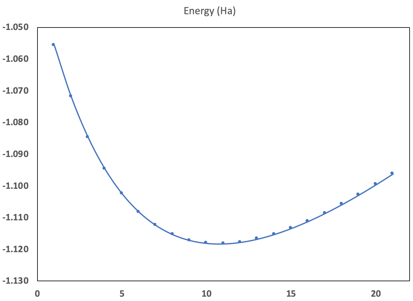
The minimum of energy in the above list is clearly between dataset 10 and 11, that is:
        xcart10   -7.2500000000E-01  0.0000000000E+00  0.0000000000E+00
                   7.2500000000E-01  0.0000000000E+00  0.0000000000E+00
        xcart11   -7.5000000000E-01  0.0000000000E+00  0.0000000000E+00
                   7.5000000000E-01  0.0000000000E+00  0.0000000000E+00
corresponding to a distance of H atoms between 1.45 Bohr and 1.50 Bohr. The forces change sign also between datasets 10 and 11:
        fcart10   -1.0358194799E-02 -0.0000000000E+00 -0.0000000000E+00
                   1.0358194799E-02 -0.0000000000E+00 -0.0000000000E+00
        fcart11    3.5571726338E-03 -0.0000000000E+00 -0.0000000000E+00
                  -3.5571726338E-03 -0.0000000000E+00 -0.0000000000E+00
From these two values, using a linear interpolation, one get the optimal value of 1.487 Bohr. Note that the number of SCF cycles drops from 6 to 5 when the wavefunctions are read from the previous dataset.
Computation of the interatomic distance (method 2)
The other methodology is based on an automatic computation of the minimum. There are different algorithms to do that. See the input variable geoopt, with values “bfgs”, “quenched”, “fire”, and “lbfgs”. In the present case, with only one degree of freedom to be optimized, the best choice is geoopt “lbfgs”.
You have also to define the maximal number of time steps for this optimization. Set the input variable ntime to 10, it will be largely enough. For the stopping criterion tolmxf, use the reasonable value of 5.0d-4 Ha/Bohr. This defines the force threshold to consider that the geometry is converged. The code will stop if the residual forces are below that value before reaching ntime.
It is also worth to change the stopping criterion for the SCF cycle, in order to be sure that the forces generated for each trial interatomic distance are sufficiently converged. Indeed, the value used for toldfe, namely 1.0d-6, might be sufficient for total energy calculations, but definitely not for the precise computation of other properties. So, change toldfe in tolrff, and set the latter input variable to 0.02. The input file tbase1_3.abi is an example of file that will do the job
# H2 molecule in a big box
#
# This file will optimize automatically the interatomic distance

#Define the methodology to find the minimum
geoopt  "bfgs"         # Use the modified Broyden algorithm
ntime   10             # Maximum number of Broyden "timesteps"
tolmxf  5.0d-4         # Stopping criterion for the geometry optimization : when
                       # the residual forces are less than tolmxf, the Broyden
                       # algorithm can stop
xcart  -0.7   0.0 0.0  # The starting values of the
        0.7   0.0 0.0  # atomic coordinates

tolrff  0.02           # Will stop the SCF cycle when, twice in a row,
                       # the ratio between the absolute maximal change of force in the SCF loop
                       # and the largest force is smaller than tolrff


nband    1             # Only one band is occupied. In order to get the energy,
                       # forces ..., there is no need to compute more than one band.

#-------------------------------------------------------------------------------
#The rest of this file is similar to the tbase1_1.in file, except
#that xcart has been moved above, and that toldfe has been replaced
#by toldff, see above.

#Definition of the unit cell
acell 10 10 10    # The keyword "acell" refers to the
                  # lengths of the primitive vectors (in Bohr)
#rprim 1 0 0  0 1 0  0 0 1 # This line, defining orthogonal primitive vectors,
                           # is commented, because it is precisely the default value of rprim

#Definition of the atom types and pseudopotentials
ntypat 1          # There is only one type of atom
znucl 1           # The keyword "znucl" refers to the atomic number of the possible type(s) of atom.
                  # Here, the only type is Hydrogen. The pseudopotential(s)
                  # mentioned after the keyword "pseudos" should correspond to this type of atom.
pp_dirpath "$ABI_PSPDIR"                 # This is the path to the directory were pseudopotentials for tests are stored
pseudos "Psdj_nc_sr_04_pw_std_psp8/H.psp8"  # Name and location of the pseudopotential
                  # This pseudopotential comes from the pseudodojo site http://www.pseudo-dojo.org/  (NC SR LDA standard),
                  # and was generated using the LDA exchange-correlation functional (PW=Perdew-Wang, ixc=-1012).
                  # By default, abinit uses the same exchange-correlation functional than the one of the input pseudopotential(s)

#Definition of the atoms
natom 2           # There are two atoms
typat 1 1         # They both are of type 1, that is, Hydrogen

#Numerical parameters of the calculation : planewave basis set and k point grid
ecut 10.0         # Maximal plane-wave kinetic energy cut-off, in Hartree
kptopt 0          # Enter the k points manually
nkpt 1            # Only one k point is needed for isolated system,
                  # taken by default to be 0.0 0.0 0.0

#Parameters for the SCF procedure
nstep 10          # Maximal number of SCF cycles
#toldfe is no more defined, as toldff is used above...
diemac 2.0        # Although this is not mandatory, it is worth to
                  # precondition the SCF cycle. The model dielectric
                  # function used as the standard preconditioner
                  # is described in the "dielng" input variable section.
                  # Here, we follow the prescriptions for molecules
                  # in a big box

##############################################################
# This section is used only for regression testing of ABINIT #
##############################################################
#%%<BEGIN TEST_INFO>
#%% [setup]
#%% executable = abinit
#%% [files]
#%% files_to_test =
#%%   tbase1_3.abo, tolnlines=  3, tolabs=  3.0e-10,   tolrel=  2.000e-08
#%% [paral_info]
#%% max_nprocs = 1
#%% [extra_info]
#%% authors = X. Gonze
#%% keywords =
#%% description =
#%%   H2 molecule in a big box
#%%   This file will optimize automatically the interatomic distance
#%%<END TEST_INFO>
while tbase1_3.abo is an example of output file:
.Version 10.5.8.2 of ABINIT, released Oct 2025.
.(MPI version, prepared for a x86_64_linux_gnu13.2 computer)

.Copyright (C) 1998-2026 ABINIT group .
 ABINIT comes with ABSOLUTELY NO WARRANTY.
 It is free software, and you are welcome to redistribute it
 under certain conditions (GNU General Public License,
 see ~abinit/COPYING or http://www.gnu.org/copyleft/gpl.txt).

 ABINIT is a project of the Universite Catholique de Louvain,
 Corning Inc. and other collaborators, see ~abinit/doc/developers/contributors.txt .
 Please read https://docs.abinit.org/theory/acknowledgments for suggested
 acknowledgments of the ABINIT effort.
 For more information, see https://www.abinit.org .

.Starting date : Sat 20 Dec 2025.
- ( at 17h05 )

- input  file    -> /home/buildbot/ABINIT3/eos_gnu_13.2_mpich/trunk__codata2022/tests/TestBot_MPI1/tutorial_tbase1_3/tbase1_3.abi
- output file    -> tbase1_3.abo
- root for input  files -> tbase1_3i
- root for output files -> tbase1_3o

 Symmetries : space group P4/m m m (#123); Bravais tP (primitive tetrag.)
================================================================================
 Values of the parameters that define the memory need of the present run
     intxc =       0    ionmov =       2      iscf =       7    lmnmax =       3
     lnmax =       3     mgfft =      30  mpssoang =       2    mqgrid =    3001
     natom =       2  nloc_mem =       1    nspden =       1   nspinor =       1
    nsppol =       1      nsym =      16    n1xccc =       0    ntypat =       1
    occopt =       1   xclevel =       1
-    mband =           1        mffmem =           1         mkmem =           1
       mpw =         752          nfft =       27000          nkpt =           1
================================================================================
P This job should need less than                       8.700 Mbytes of memory.
  Rough estimation (10% accuracy) of disk space for files :
_ WF disk file :      0.013 Mbytes ; DEN or POT disk file :      0.208 Mbytes.
================================================================================

--------------------------------------------------------------------------------
------------- Echo of variables that govern the present computation ------------
--------------------------------------------------------------------------------
-
- outvars: echo of selected default values
-   iomode0 =  0 , fftalg0 =512 , wfoptalg0 =  0
-
- outvars: echo of global parameters not present in the input file
-  max_nthreads =    0
-
 -outvars: echo values of preprocessed input variables --------
            acell      1.0000000000E+01  1.0000000000E+01  1.0000000000E+01 Bohr
              amu      1.00794000E+00
           diemac      2.00000000E+00
             ecut      1.00000000E+01 Hartree
-          fftalg         512
           ionmov           2
           istwfk        2
              ixc       -1012
           kptopt           0
P           mkmem           1
            natom           2
            nband           1
            ngfft          30      30      30
             nkpt           1
            nstep          10
             nsym          16
            ntime          10
           ntypat           1
              occ      2.000000
        optforces           1
          spgroup         123
           symrel      1  0  0   0  1  0   0  0  1      -1  0  0   0 -1  0   0  0 -1
                      -1  0  0   0  1  0   0  0 -1       1  0  0   0 -1  0   0  0  1
                      -1  0  0   0 -1  0   0  0  1       1  0  0   0  1  0   0  0 -1
                       1  0  0   0 -1  0   0  0 -1      -1  0  0   0  1  0   0  0  1
                       1  0  0   0  0  1   0  1  0      -1  0  0   0  0 -1   0 -1  0
                      -1  0  0   0  0  1   0 -1  0       1  0  0   0  0 -1   0  1  0
                      -1  0  0   0  0 -1   0  1  0       1  0  0   0  0  1   0 -1  0
                       1  0  0   0  0 -1   0 -1  0      -1  0  0   0  0  1   0  1  0
           tolmxf      5.00000000E-04
           tolrff      2.00000000E-02
            typat      1  1
           xangst     -3.7042404738E-01  0.0000000000E+00  0.0000000000E+00
                       3.7042404738E-01  0.0000000000E+00  0.0000000000E+00
            xcart     -7.0000000000E-01  0.0000000000E+00  0.0000000000E+00
                       7.0000000000E-01  0.0000000000E+00  0.0000000000E+00
             xred     -7.0000000000E-02  0.0000000000E+00  0.0000000000E+00
                       7.0000000000E-02  0.0000000000E+00  0.0000000000E+00
            znucl        1.00000

================================================================================

 chkinp: Checking input parameters for consistency.

================================================================================
== DATASET  1 ==================================================================
-   mpi_nproc: 1, omp_nthreads: -1 (-1 if OMP is not activated)


--- !DatasetInfo
iteration_state: {dtset: 1, }
dimensions: {natom: 2, nkpt: 1, mband: 1, nsppol: 1, nspinor: 1, nspden: 1, mpw: 752, }
cutoff_energies: {ecut:  10.0, pawecutdg:  -1.0, }
electrons: {nelect:   2.00000000E+00, charge:   0.00000000E+00, occopt:   1.00000000E+00, tsmear:   1.00000000E-02, }
meta: {optdriver: 0, ionmov: 2, optcell: 0, iscf: 7, paral_kgb: 0, }
...

 Real(R)+Recip(G) space primitive vectors, cartesian coordinates (Bohr,Bohr^-1):
 R(1)= 10.0000000  0.0000000  0.0000000  G(1)=  0.1000000  0.0000000  0.0000000
 R(2)=  0.0000000 10.0000000  0.0000000  G(2)=  0.0000000  0.1000000  0.0000000
 R(3)=  0.0000000  0.0000000 10.0000000  G(3)=  0.0000000  0.0000000  0.1000000
 Unit cell volume ucvol=  1.0000000E+03 bohr^3
 Angles (23,13,12)=  9.00000000E+01  9.00000000E+01  9.00000000E+01 degrees

 getcut: wavevector=  0.0000  0.0000  0.0000  ngfft=  30  30  30
         ecut(hartree)=     10.000   => boxcut(ratio)=   2.10744

--- Pseudopotential description ------------------------------------------------
- pspini: atom type   1  psp file is /home/buildbot/ABINIT3/eos_gnu_13.2_mpich/trunk__codata2022/tests/Pspdir/Psdj_nc_sr_04_pw_std_psp8/H.psp8
- pspatm: opening atomic psp file    /home/buildbot/ABINIT3/eos_gnu_13.2_mpich/trunk__codata2022/tests/Pspdir/Psdj_nc_sr_04_pw_std_psp8/H.psp8
- H     ONCVPSP-3.3.0  r_core=   1.00957   0.90680
-  1.00000   1.00000    171101                znucl, zion, pspdat
    8   -1012    1    4       300   0.00000   pspcod,pspxc,lmax,lloc,mmax,r2well
    2.99000000000000    0.00000000000000    0.00000000000000   rchrg,fchrg,qchrg
     nproj     2     1
     extension_switch     1
  pspatm : epsatm=    0.35491505
         --- l  ekb(1:nproj) -->
             0   -1.665338   -0.519510
             1   -0.275071
 pspatm: atomic psp has been read  and splines computed

   1.41966018E+00                                ecore*ucvol(ha*bohr**3)
--------------------------------------------------------------------------------

_setup2: Arith. and geom. avg. npw (full set) are    1503.000    1503.000

================================================================================

=== [ionmov= 2] Broyden-Fletcher-Goldfarb-Shanno method (forces)
================================================================================

--- Iteration: ( 1/10) Internal Cycle: (1/1)
--------------------------------------------------------------------------------

---SELF-CONSISTENT-FIELD CONVERGENCE--------------------------------------------

--- !BeginCycle
iteration_state: {dtset: 1, itime: 1, icycle: 1, }
solver: {iscf: 7, nstep: 10, nline: 4, wfoptalg: 0, }
tolerances: {tolrff: 2.00E-02, }
...

     iter   Etot(hartree)      deltaE(h)  residm     vres2    diffor    maxfor
 ETOT  1  -1.1094662760139    -1.109E+00 2.634E-06 1.742E+01 1.649E-03 1.649E-03
 ETOT  2  -1.1170451552865    -7.579E-03 1.569E-09 2.639E-01 3.140E-02 2.975E-02
 ETOT  3  -1.1171734568401    -1.283E-04 9.871E-07 6.721E-02 3.910E-03 2.584E-02
 ETOT  4  -1.1171842840515    -1.083E-05 5.933E-08 6.908E-04 1.127E-03 2.697E-02
 ETOT  5  -1.1171843456996    -6.165E-08 2.922E-11 9.525E-06 5.475E-05 2.691E-02
 ETOT  6  -1.1171843463486    -6.490E-10 1.734E-12 3.695E-07 1.013E-05 2.690E-02

 At SCF step    6, forces are sufficiently converged :
  for the second time, max diff in force=  1.013E-05 is less than < tolrff=  2.000E-02 times max force

 Cartesian components of stress tensor (hartree/bohr^3)
  sigma(1 1)= -3.33755106E-06  sigma(3 2)=  0.00000000E+00
  sigma(2 2)=  3.45785448E-05  sigma(3 1)=  0.00000000E+00
  sigma(3 3)=  3.45785448E-05  sigma(2 1)=  0.00000000E+00


--- !ResultsGS
iteration_state: {dtset: 1, itime: 1, icycle: 1, }
comment   : Summary of ground state results
lattice_vectors:
- [ 10.0000000,   0.0000000,   0.0000000, ]
- [  0.0000000,  10.0000000,   0.0000000, ]
- [  0.0000000,   0.0000000,  10.0000000, ]
lattice_lengths: [  10.00000,   10.00000,   10.00000, ]
lattice_angles: [ 90.000,  90.000,  90.000, ] # degrees, (23, 13, 12)
lattice_volume:   1.0000000E+03
convergence: {deltae: -6.490E-10, res2:  3.695E-07, residm:  1.734E-12, diffor:  1.013E-05, }
etotal    :  -1.11718435E+00
entropy   :   0.00000000E+00
fermie    :  -3.69424887E-01
cartesian_stress_tensor: # hartree/bohr^3
- [ -3.33755106E-06,   0.00000000E+00,   0.00000000E+00, ]
- [  0.00000000E+00,   3.45785448E-05,   0.00000000E+00, ]
- [  0.00000000E+00,   0.00000000E+00,   3.45785448E-05, ]
pressure_GPa:  -6.4549E-01
xred      :
- [ -7.0000E-02,   0.0000E+00,   0.0000E+00,  H]
- [  7.0000E-02,   0.0000E+00,   0.0000E+00,  H]
cartesian_forces: # hartree/bohr
- [ -2.69019375E-02,  -0.00000000E+00,  -0.00000000E+00, ]
- [  2.69019375E-02,  -0.00000000E+00,  -0.00000000E+00, ]
force_length_stats: {min:   2.69019375E-02, max:   2.69019375E-02, mean:   2.69019375E-02, }
...

 Integrated electronic density in atomic spheres:
 ------------------------------------------------
 Atom  Sphere_radius  Integrated_density
    1        2.00000          1.44870400
    2        2.00000          1.44870400

---OUTPUT-----------------------------------------------------------------------

 Cartesian coordinates (xcart) [bohr]
 -7.00000000000000E-01  0.00000000000000E+00  0.00000000000000E+00
  7.00000000000000E-01  0.00000000000000E+00  0.00000000000000E+00
 Reduced coordinates (xred)
 -7.00000000000000E-02  0.00000000000000E+00  0.00000000000000E+00
  7.00000000000000E-02  0.00000000000000E+00  0.00000000000000E+00
 Cartesian forces (fcart) [Ha/bohr]; max,rms= 2.69019E-02 1.55318E-02 (free atoms)
 -2.69019375251367E-02 -0.00000000000000E+00 -0.00000000000000E+00
  2.69019375251367E-02 -0.00000000000000E+00 -0.00000000000000E+00
 Gradient of E wrt nuclear positions in reduced coordinates (gred)
  2.69019375251367E-01  0.00000000000000E+00  0.00000000000000E+00
 -2.69019375251367E-01 -0.00000000000000E+00 -0.00000000000000E+00
 Total energy (etotal) [Ha]= -1.11718434634860E+00

--- Iteration: ( 2/10) Internal Cycle: (1/1)
--------------------------------------------------------------------------------

---SELF-CONSISTENT-FIELD CONVERGENCE--------------------------------------------

--- !BeginCycle
iteration_state: {dtset: 1, itime: 2, icycle: 1, }
solver: {iscf: 7, nstep: 10, nline: 4, wfoptalg: 0, }
tolerances: {tolrff: 2.00E-02, }
...

     iter   Etot(hartree)      deltaE(h)  residm     vres2    diffor    maxfor
 ETOT  1  -1.1181341236636    -1.118E+00 1.241E-10 2.637E-02 1.762E-02 9.279E-03
 ETOT  2  -1.1181408029217    -6.679E-06 1.460E-12 7.011E-04 1.850E-04 9.094E-03
 ETOT  3  -1.1181409536076    -1.507E-07 1.295E-09 1.267E-04 1.571E-04 9.251E-03
 ETOT  4  -1.1181409705200    -1.691E-08 9.301E-11 2.737E-06 3.907E-05 9.212E-03

 At SCF step    4, forces are sufficiently converged :
  for the second time, max diff in force=  3.907E-05 is less than < tolrff=  2.000E-02 times max force

 Cartesian components of stress tensor (hartree/bohr^3)
  sigma(1 1)=  2.38241397E-05  sigma(3 2)=  0.00000000E+00
  sigma(2 2)=  3.38218937E-05  sigma(3 1)=  0.00000000E+00
  sigma(3 3)=  3.38218937E-05  sigma(2 1)=  0.00000000E+00


--- !ResultsGS
iteration_state: {dtset: 1, itime: 2, icycle: 1, }
comment   : Summary of ground state results
lattice_vectors:
- [ 10.0000000,   0.0000000,   0.0000000, ]
- [  0.0000000,  10.0000000,   0.0000000, ]
- [  0.0000000,   0.0000000,  10.0000000, ]
lattice_lengths: [  10.00000,   10.00000,   10.00000, ]
lattice_angles: [ 90.000,  90.000,  90.000, ] # degrees, (23, 13, 12)
lattice_volume:   1.0000000E+03
convergence: {deltae: -1.691E-08, res2:  2.737E-06, residm:  9.301E-11, diffor:  3.907E-05, }
etotal    :  -1.11814097E+00
entropy   :   0.00000000E+00
fermie    :  -3.64719629E-01
cartesian_stress_tensor: # hartree/bohr^3
- [  2.38241397E-05,   0.00000000E+00,   0.00000000E+00, ]
- [  0.00000000E+00,   3.38218937E-05,   0.00000000E+00, ]
- [  0.00000000E+00,   0.00000000E+00,   3.38218937E-05, ]
pressure_GPa:  -8.9703E-01
xred      :
- [ -7.2690E-02,   0.0000E+00,   0.0000E+00,  H]
- [  7.2690E-02,   0.0000E+00,   0.0000E+00,  H]
cartesian_forces: # hartree/bohr
- [ -9.21224104E-03,  -0.00000000E+00,  -0.00000000E+00, ]
- [  9.21224104E-03,  -0.00000000E+00,  -0.00000000E+00, ]
force_length_stats: {min:   9.21224104E-03, max:   9.21224104E-03, mean:   9.21224104E-03, }
...

 Integrated electronic density in atomic spheres:
 ------------------------------------------------
 Atom  Sphere_radius  Integrated_density
    1        2.00000          1.42693450
    2        2.00000          1.42693450

---OUTPUT-----------------------------------------------------------------------

 Cartesian coordinates (xcart) [bohr]
 -7.26901937525137E-01  0.00000000000000E+00  0.00000000000000E+00
  7.26901937525137E-01  0.00000000000000E+00  0.00000000000000E+00
 Reduced coordinates (xred)
 -7.26901937525137E-02  0.00000000000000E+00  0.00000000000000E+00
  7.26901937525137E-02  0.00000000000000E+00  0.00000000000000E+00
 Cartesian forces (fcart) [Ha/bohr]; max,rms= 9.21224E-03 5.31869E-03 (free atoms)
 -9.21224103518608E-03 -0.00000000000000E+00 -0.00000000000000E+00
  9.21224103518608E-03 -0.00000000000000E+00 -0.00000000000000E+00
 Gradient of E wrt nuclear positions in reduced coordinates (gred)
  9.21224103518608E-02  0.00000000000000E+00  0.00000000000000E+00
 -9.21224103518608E-02 -0.00000000000000E+00 -0.00000000000000E+00
 Total energy (etotal) [Ha]= -1.11814097051997E+00

 Difference of energy with previous step (new-old):
           Absolute (Ha)=-9.56624E-04
           Relative     =-8.55915E-04

--- Iteration: ( 3/10) Internal Cycle: (1/1)
--------------------------------------------------------------------------------

---SELF-CONSISTENT-FIELD CONVERGENCE--------------------------------------------

--- !BeginCycle
iteration_state: {dtset: 1, itime: 3, icycle: 1, }
solver: {iscf: 7, nstep: 10, nline: 4, wfoptalg: 0, }
tolerances: {tolrff: 2.00E-02, }
...

     iter   Etot(hartree)      deltaE(h)  residm     vres2    diffor    maxfor
 ETOT  1  -1.1182837181775    -1.118E+00 3.402E-11 7.018E-03 7.950E-03 1.262E-03
 ETOT  2  -1.1182854751204    -1.757E-06 3.783E-13 1.843E-04 9.169E-05 1.171E-03
 ETOT  3  -1.1182855140288    -3.891E-08 3.322E-10 3.309E-05 7.828E-05 1.249E-03
 ETOT  4  -1.1182855183094    -4.281E-09 2.352E-11 7.304E-07 1.916E-05 1.230E-03
 ETOT  5  -1.1182855183625    -5.314E-11 4.421E-14 1.157E-08 1.112E-06 1.231E-03

 At SCF step    5, forces are sufficiently converged :
  for the second time, max diff in force=  1.112E-06 is less than < tolrff=  2.000E-02 times max force

 Cartesian components of stress tensor (hartree/bohr^3)
  sigma(1 1)=  3.67494741E-05  sigma(3 2)=  0.00000000E+00
  sigma(2 2)=  3.35327287E-05  sigma(3 1)=  0.00000000E+00
  sigma(3 3)=  3.35327287E-05  sigma(2 1)=  0.00000000E+00


--- !ResultsGS
iteration_state: {dtset: 1, itime: 3, icycle: 1, }
comment   : Summary of ground state results
lattice_vectors:
- [ 10.0000000,   0.0000000,   0.0000000, ]
- [  0.0000000,  10.0000000,   0.0000000, ]
- [  0.0000000,   0.0000000,  10.0000000, ]
lattice_lengths: [  10.00000,   10.00000,   10.00000, ]
lattice_angles: [ 90.000,  90.000,  90.000, ] # degrees, (23, 13, 12)
lattice_volume:   1.0000000E+03
convergence: {deltae: -5.314E-11, res2:  1.157E-08, residm:  4.421E-14, diffor:  1.112E-06, }
etotal    :  -1.11828552E+00
entropy   :   0.00000000E+00
fermie    :  -3.62339980E-01
cartesian_stress_tensor: # hartree/bohr^3
- [  3.67494741E-05,   0.00000000E+00,   0.00000000E+00, ]
- [  0.00000000E+00,   3.35327287E-05,   0.00000000E+00, ]
- [  0.00000000E+00,   0.00000000E+00,   3.35327287E-05, ]
pressure_GPa:  -1.0181E+00
xred      :
- [ -7.4091E-02,   0.0000E+00,   0.0000E+00,  H]
- [  7.4091E-02,   0.0000E+00,   0.0000E+00,  H]
cartesian_forces: # hartree/bohr
- [ -1.23077796E-03,  -0.00000000E+00,  -0.00000000E+00, ]
- [  1.23077796E-03,  -0.00000000E+00,  -0.00000000E+00, ]
force_length_stats: {min:   1.23077796E-03, max:   1.23077796E-03, mean:   1.23077796E-03, }
...

 Integrated electronic density in atomic spheres:
 ------------------------------------------------
 Atom  Sphere_radius  Integrated_density
    1        2.00000          1.41202881
    2        2.00000          1.41202881

---OUTPUT-----------------------------------------------------------------------

 Cartesian coordinates (xcart) [bohr]
 -7.40911625760085E-01  0.00000000000000E+00  0.00000000000000E+00
  7.40911625760085E-01  0.00000000000000E+00  0.00000000000000E+00
 Reduced coordinates (xred)
 -7.40911625760085E-02  0.00000000000000E+00  0.00000000000000E+00
  7.40911625760085E-02  0.00000000000000E+00  0.00000000000000E+00
 Cartesian forces (fcart) [Ha/bohr]; max,rms= 1.23078E-03 7.10590E-04 (free atoms)
 -1.23077795517666E-03 -0.00000000000000E+00 -0.00000000000000E+00
  1.23077795517666E-03 -0.00000000000000E+00 -0.00000000000000E+00
 Gradient of E wrt nuclear positions in reduced coordinates (gred)
  1.23077795517666E-02  0.00000000000000E+00  0.00000000000000E+00
 -1.23077795517666E-02 -0.00000000000000E+00 -0.00000000000000E+00
 Total energy (etotal) [Ha]= -1.11828551836253E+00

 Difference of energy with previous step (new-old):
           Absolute (Ha)=-1.44548E-04
           Relative     =-1.29267E-04

--- Iteration: ( 4/10) Internal Cycle: (1/1)
--------------------------------------------------------------------------------

---SELF-CONSISTENT-FIELD CONVERGENCE--------------------------------------------

--- !BeginCycle
iteration_state: {dtset: 1, itime: 4, icycle: 1, }
solver: {iscf: 7, nstep: 10, nline: 4, wfoptalg: 0, }
tolerances: {tolrff: 2.00E-02, }
...

     iter   Etot(hartree)      deltaE(h)  residm     vres2    diffor    maxfor
 ETOT  1  -1.1182882719785    -1.118E+00 7.783E-13 1.636E-04 1.159E-03 7.217E-05
 ETOT  2  -1.1182883127945    -4.082E-08 8.627E-15 4.264E-06 1.536E-05 5.682E-05
 ETOT  3  -1.1182883137014    -9.069E-10 7.711E-12 7.663E-07 1.193E-05 6.875E-05
 ETOT  4  -1.1182883137993    -9.791E-11 5.391E-13 1.744E-08 2.879E-06 6.587E-05
 ETOT  5  -1.1182883138008    -1.428E-12 1.038E-15 2.642E-10 1.697E-07 6.604E-05
 ETOT  6  -1.1182883138007     1.210E-13 2.667E-18 6.445E-12 7.190E-09 6.603E-05

 At SCF step    6, forces are sufficiently converged :
  for the second time, max diff in force=  7.190E-09 is less than < tolrff=  2.000E-02 times max force

 Cartesian components of stress tensor (hartree/bohr^3)
  sigma(1 1)=  3.86729261E-05  sigma(3 2)=  0.00000000E+00
  sigma(2 2)=  3.34916913E-05  sigma(3 1)=  0.00000000E+00
  sigma(3 3)=  3.34916913E-05  sigma(2 1)=  0.00000000E+00


--- !ResultsGS
iteration_state: {dtset: 1, itime: 4, icycle: 1, }
comment   : Summary of ground state results
lattice_vectors:
- [ 10.0000000,   0.0000000,   0.0000000, ]
- [  0.0000000,  10.0000000,   0.0000000, ]
- [  0.0000000,   0.0000000,  10.0000000, ]
lattice_lengths: [  10.00000,   10.00000,   10.00000, ]
lattice_angles: [ 90.000,  90.000,  90.000, ] # degrees, (23, 13, 12)
lattice_volume:   1.0000000E+03
convergence: {deltae:  1.210E-13, res2:  6.445E-12, residm:  2.667E-18, diffor:  7.190E-09, }
etotal    :  -1.11828831E+00
entropy   :   0.00000000E+00
fermie    :  -3.61980956E-01
cartesian_stress_tensor: # hartree/bohr^3
- [  3.86729261E-05,   0.00000000E+00,   0.00000000E+00, ]
- [  0.00000000E+00,   3.34916913E-05,   0.00000000E+00, ]
- [  0.00000000E+00,   0.00000000E+00,   3.34916913E-05, ]
pressure_GPa:  -1.0362E+00
xred      :
- [ -7.4307E-02,   0.0000E+00,   0.0000E+00,  H]
- [  7.4307E-02,   0.0000E+00,   0.0000E+00,  H]
cartesian_forces: # hartree/bohr
- [ -6.60322237E-05,  -0.00000000E+00,  -0.00000000E+00, ]
- [  6.60322237E-05,  -0.00000000E+00,  -0.00000000E+00, ]
force_length_stats: {min:   6.60322237E-05, max:   6.60322237E-05, mean:   6.60322237E-05, }
...

 Integrated electronic density in atomic spheres:
 ------------------------------------------------
 Atom  Sphere_radius  Integrated_density
    1        2.00000          1.41060988
    2        2.00000          1.41060988

---OUTPUT-----------------------------------------------------------------------

 Cartesian coordinates (xcart) [bohr]
 -7.43071983487187E-01  0.00000000000000E+00  0.00000000000000E+00
  7.43071983487187E-01  0.00000000000000E+00  0.00000000000000E+00
 Reduced coordinates (xred)
 -7.43071983487187E-02  0.00000000000000E+00  0.00000000000000E+00
  7.43071983487187E-02  0.00000000000000E+00  0.00000000000000E+00
 Cartesian forces (fcart) [Ha/bohr]; max,rms= 6.60322E-05 3.81237E-05 (free atoms)
 -6.60322237264216E-05 -0.00000000000000E+00 -0.00000000000000E+00
  6.60322237264216E-05 -0.00000000000000E+00 -0.00000000000000E+00
 Gradient of E wrt nuclear positions in reduced coordinates (gred)
  6.60322237264216E-04  0.00000000000000E+00  0.00000000000000E+00
 -6.60322237264216E-04 -0.00000000000000E+00 -0.00000000000000E+00
 Total energy (etotal) [Ha]= -1.11828831380065E+00

 Difference of energy with previous step (new-old):
           Absolute (Ha)=-2.79544E-06
           Relative     =-2.49975E-06

 At Broyd/MD step   4, gradients are converged :
  max grad (force/stress) = 6.6032E-05 < tolmxf= 5.0000E-04 ha/bohr (free atoms)

================================================================================

 ----iterations are completed or convergence reached----

 Mean square residual over all n,k,spin=   26.667E-19; max=  26.667E-19
 reduced coordinates (array xred) for    2 atoms
      -0.074307198349      0.000000000000      0.000000000000
       0.074307198349      0.000000000000      0.000000000000
 rms dE/dt=  3.8124E-04; max dE/dt=  6.6032E-04; dE/dt below (all hartree)
    1       0.000660322237      0.000000000000      0.000000000000
    2      -0.000660322237      0.000000000000      0.000000000000

 cartesian coordinates (angstrom) at end:
    1     -0.39321675945515     0.00000000000000     0.00000000000000
    2      0.39321675945515     0.00000000000000     0.00000000000000

 cartesian forces (hartree/bohr) at end:
    1     -0.00006603222373    -0.00000000000000    -0.00000000000000
    2      0.00006603222373    -0.00000000000000    -0.00000000000000
 frms,max,avg= 3.8123722E-05 6.6032224E-05   0.000E+00  0.000E+00  0.000E+00 h/b

 cartesian forces (eV/Angstrom) at end:
    1     -0.00339551346637    -0.00000000000000    -0.00000000000000
    2      0.00339551346637    -0.00000000000000    -0.00000000000000
 frms,max,avg= 1.9604006E-03 3.3955135E-03   0.000E+00  0.000E+00  0.000E+00 e/A
 length scales= 10.000000000000 10.000000000000 10.000000000000 bohr
              =  5.291772105440  5.291772105440  5.291772105440 angstroms
 prteigrs : about to open file tbase1_3o_EIG
 Fermi (or HOMO) energy (hartree) =  -0.36198   Average Vxc (hartree)=  -0.07525
 Eigenvalues (hartree) for nkpt=   1  k points:
 kpt#   1, nband=  1, wtk=  1.00000, kpt=  0.0000  0.0000  0.0000 (reduced coord)
  -0.36198

--- !EnergyTerms
iteration_state     : {dtset: 1, itime: 4, icycle: 1, }
comment             : Components of total free energy in Hartree
kinetic             :  9.77513704261900E-01
hartree             :  6.97324256766169E-01
xc                  : -6.25836844129810E-01
Ewald energy        :  1.10200870637778E-01
psp_core            :  1.41966018330111E-03
local_psp           : -2.12634774954400E+00
non_local_psp       : -1.52562211975992E-01
total_energy        : -1.11828831380065E+00
total_energy_eV     : -3.04301752411964E+01
band_energy         : -7.23961912630883E-01
...

 rms coord change=  2.4868E-03   atom, delta coord (reduced):
     1       -0.004307198349      0.000000000000      0.000000000000
     2        0.004307198349      0.000000000000      0.000000000000

 Cartesian components of stress tensor (hartree/bohr^3)
  sigma(1 1)=  3.86729261E-05  sigma(3 2)=  0.00000000E+00
  sigma(2 2)=  3.34916913E-05  sigma(3 1)=  0.00000000E+00
  sigma(3 3)=  3.34916913E-05  sigma(2 1)=  0.00000000E+00

-Cartesian components of stress tensor (GPa)         [Pressure= -1.0362E+00 GPa]
- sigma(1 1)=  1.13779677E+00  sigma(3 2)=  0.00000000E+00
- sigma(2 2)=  9.85359578E-01  sigma(3 1)=  0.00000000E+00
- sigma(3 3)=  9.85359578E-01  sigma(2 1)=  0.00000000E+00

== END DATASET(S) ==============================================================
================================================================================

 -outvars: echo values of variables after computation  --------
            acell      1.0000000000E+01  1.0000000000E+01  1.0000000000E+01 Bohr
              amu      1.00794000E+00
           diemac      2.00000000E+00
             ecut      1.00000000E+01 Hartree
           etotal     -1.1182883138E+00
            fcart     -6.6032223726E-05 -0.0000000000E+00 -0.0000000000E+00
                       6.6032223726E-05 -0.0000000000E+00 -0.0000000000E+00
-          fftalg         512
           ionmov           2
           istwfk        2
              ixc       -1012
           kptopt           0
P           mkmem           1
            natom           2
            nband           1
            ngfft          30      30      30
             nkpt           1
            nstep          10
             nsym          16
            ntime          10
           ntypat           1
              occ      2.000000
        optforces           1
          spgroup         123
           strten      3.8672926053E-05  3.3491691335E-05  3.3491691335E-05
                       0.0000000000E+00  0.0000000000E+00  0.0000000000E+00
           symrel      1  0  0   0  1  0   0  0  1      -1  0  0   0 -1  0   0  0 -1
                      -1  0  0   0  1  0   0  0 -1       1  0  0   0 -1  0   0  0  1
                      -1  0  0   0 -1  0   0  0  1       1  0  0   0  1  0   0  0 -1
                       1  0  0   0 -1  0   0  0 -1      -1  0  0   0  1  0   0  0  1
                       1  0  0   0  0  1   0  1  0      -1  0  0   0  0 -1   0 -1  0
                      -1  0  0   0  0  1   0 -1  0       1  0  0   0  0 -1   0  1  0
                      -1  0  0   0  0 -1   0  1  0       1  0  0   0  0  1   0 -1  0
                       1  0  0   0  0 -1   0 -1  0      -1  0  0   0  0  1   0  1  0
           tolmxf      5.00000000E-04
           tolrff      2.00000000E-02
            typat      1  1
           xangst     -3.9321675946E-01  0.0000000000E+00  0.0000000000E+00
                       3.9321675946E-01  0.0000000000E+00  0.0000000000E+00
            xcart     -7.4307198349E-01  0.0000000000E+00  0.0000000000E+00
                       7.4307198349E-01  0.0000000000E+00  0.0000000000E+00
             xred     -7.4307198349E-02  0.0000000000E+00  0.0000000000E+00
                       7.4307198349E-02  0.0000000000E+00  0.0000000000E+00
            znucl        1.00000

================================================================================


- Timing analysis has been suppressed with timopt=0


================================================================================

 Suggested references for the acknowledgment of ABINIT usage.

 The users of ABINIT have little formal obligations with respect to the ABINIT group
 (those specified in the GNU General Public License, http://www.gnu.org/copyleft/gpl.txt).
 However, it is common practice in the scientific literature,
 to acknowledge the efforts of people that have made the research possible.
 In this spirit, please find below suggested citations of work written by ABINIT developers,
 corresponding to implementations inside of ABINIT that you have used in the present run.
 Note also that it will be of great value to readers of publications presenting these results,
 to read papers enabling them to understand the theoretical formalism and details
 of the ABINIT implementation.
 For information on why they are suggested, see also https://docs.abinit.org/theory/acknowledgments.
-
- [1] Libxc: A library of exchange and correlation functionals for density functional theory.
- M.A.L. Marques, M.J.T. Oliveira, T. Burnus, Computer Physics Communications 183, 2227 (2012).
- Comment: to be cited when LibXC is used (negative value of ixc)
- Strong suggestion to cite this paper.
- DOI and bibtex: see https://docs.abinit.org/theory/bibliography/#marques2012
-
- [2] The Abinit project: Impact, environment and recent developments.
- Computer Phys. Comm. 248, 107042 (2020).
- X.Gonze, B. Amadon, G. Antonius, F.Arnardi, L.Baguet, J.-M.Beuken,
- J.Bieder, F.Bottin, J.Bouchet, E.Bousquet, N.Brouwer, F.Bruneval,
- G.Brunin, T.Cavignac, J.-B. Charraud, Wei Chen, M.Cote, S.Cottenier,
- J.Denier, G.Geneste, Ph.Ghosez, M.Giantomassi, Y.Gillet, O.Gingras,
- D.R.Hamann, G.Hautier, Xu He, N.Helbig, N.Holzwarth, Y.Jia, F.Jollet,
- W.Lafargue-Dit-Hauret, K.Lejaeghere, M.A.L.Marques, A.Martin, C.Martins,
- H.P.C. Miranda, F.Naccarato, K. Persson, G.Petretto, V.Planes, Y.Pouillon,
- S.Prokhorenko, F.Ricci, G.-M.Rignanese, A.H.Romero, M.M.Schmitt, M.Torrent,
- M.J.van Setten, B.Van Troeye, M.J.Verstraete, G.Zerah and J.W.Zwanzig
- Comment: the fifth generic paper describing the ABINIT project.
- Note that a version of this paper, that is not formatted for Computer Phys. Comm.
- is available at https://www.abinit.org/sites/default/files/ABINIT20.pdf .
- The licence allows the authors to put it on the Web.
- DOI and bibtex: see https://docs.abinit.org/theory/bibliography/#gonze2020
-
- [3] Optimized norm-conserving Vanderbilt pseudopotentials.
- D.R. Hamann, Phys. Rev. B 88, 085117 (2013).
- Comment: Some pseudopotential generated using the ONCVPSP code were used.
- DOI and bibtex: see https://docs.abinit.org/theory/bibliography/#hamann2013
-
- [4] ABINIT: Overview, and focus on selected capabilities
- J. Chem. Phys. 152, 124102 (2020).
- A. Romero, D.C. Allan, B. Amadon, G. Antonius, T. Applencourt, L.Baguet,
- J.Bieder, F.Bottin, J.Bouchet, E.Bousquet, F.Bruneval,
- G.Brunin, D.Caliste, M.Cote,
- J.Denier, C. Dreyer, Ph.Ghosez, M.Giantomassi, Y.Gillet, O.Gingras,
- D.R.Hamann, G.Hautier, F.Jollet, G. Jomard,
- A.Martin,
- H.P.C. Miranda, F.Naccarato, G.Petretto, N.A. Pike, V.Planes,
- S.Prokhorenko, T. Rangel, F.Ricci, G.-M.Rignanese, M.Royo, M.Stengel, M.Torrent,
- M.J.van Setten, B.Van Troeye, M.J.Verstraete, J.Wiktor, J.W.Zwanziger, and X.Gonze.
- Comment: a global overview of ABINIT, with focus on selected capabilities .
- Note that a version of this paper, that is not formatted for J. Chem. Phys
- is available at https://www.abinit.org/sites/default/files/ABINIT20_JPC.pdf .
- The licence allows the authors to put it on the Web.
- DOI and bibtex: see https://docs.abinit.org/theory/bibliography/#romero2020
-
- [5] Recent developments in the ABINIT software package.
- Computer Phys. Comm. 205, 106 (2016).
- X.Gonze, F.Jollet, F.Abreu Araujo, D.Adams, B.Amadon, T.Applencourt,
- C.Audouze, J.-M.Beuken, J.Bieder, A.Bokhanchuk, E.Bousquet, F.Bruneval
- D.Caliste, M.Cote, F.Dahm, F.Da Pieve, M.Delaveau, M.Di Gennaro,
- B.Dorado, C.Espejo, G.Geneste, L.Genovese, A.Gerossier, M.Giantomassi,
- Y.Gillet, D.R.Hamann, L.He, G.Jomard, J.Laflamme Janssen, S.Le Roux,
- A.Levitt, A.Lherbier, F.Liu, I.Lukacevic, A.Martin, C.Martins,
- M.J.T.Oliveira, S.Ponce, Y.Pouillon, T.Rangel, G.-M.Rignanese,
- A.H.Romero, B.Rousseau, O.Rubel, A.A.Shukri, M.Stankovski, M.Torrent,
- M.J.Van Setten, B.Van Troeye, M.J.Verstraete, D.Waroquier, J.Wiktor,
- B.Xu, A.Zhou, J.W.Zwanziger.
- Comment: the fourth generic paper describing the ABINIT project.
- Note that a version of this paper, that is not formatted for Computer Phys. Comm.
- is available at https://www.abinit.org/sites/default/files/ABINIT16.pdf .
- The licence allows the authors to put it on the Web.
- DOI and bibtex: see https://docs.abinit.org/theory/bibliography/#gonze2016
-
- Proc.   0 individual time (sec): cpu=          0.8  wall=          0.9

================================================================================

 Calculation completed.
.Delivered  22 WARNINGs and   4 COMMENTs to log file.
+Overall time at end (sec) : cpu=          0.8  wall=          0.9
So, you run the code with your input file (a few seconds), examine quietly this file (which is much smaller than the tbase1_2.abo file), and get some significant output data gathered in the final echo of variables:
       etotal     -1.1182883138E+00
        fcart     -6.6032223725E-05 -0.0000000000E+00 -0.0000000000E+00
                   6.6032223725E-05 -0.0000000000E+00 -0.0000000000E+00
         ...
        xcart     -7.4307198349E-01  0.0000000000E+00  0.0000000000E+00
                   7.4307198349E-01  0.0000000000E+00  0.0000000000E+00
According to these data (see xcart), the optimal interatomic distance is about 1.486 Bohr, in good agreement with the estimation of tbase1_2.abo. If you have time (this is to be done at home), you might try to change the stopping criteria, and redo the calculation, to see the level of convergence of the interatomic distance.
Note that the final value of fcart in your run might differ slightly from the one shown above (less than one percent change). Such a fluctuation is quite often observed for a value converging to zero (remember, we ask the code to determine the equilibrium geometry, that is, forces should be zero) when the same computation is done on different platforms.
Tip
With AbiPy , we can analyze easily the results of the structural relaxation with the abiopen.py script:
abiopen.py tbase1_3o_HIST.nc --expose --seaborn
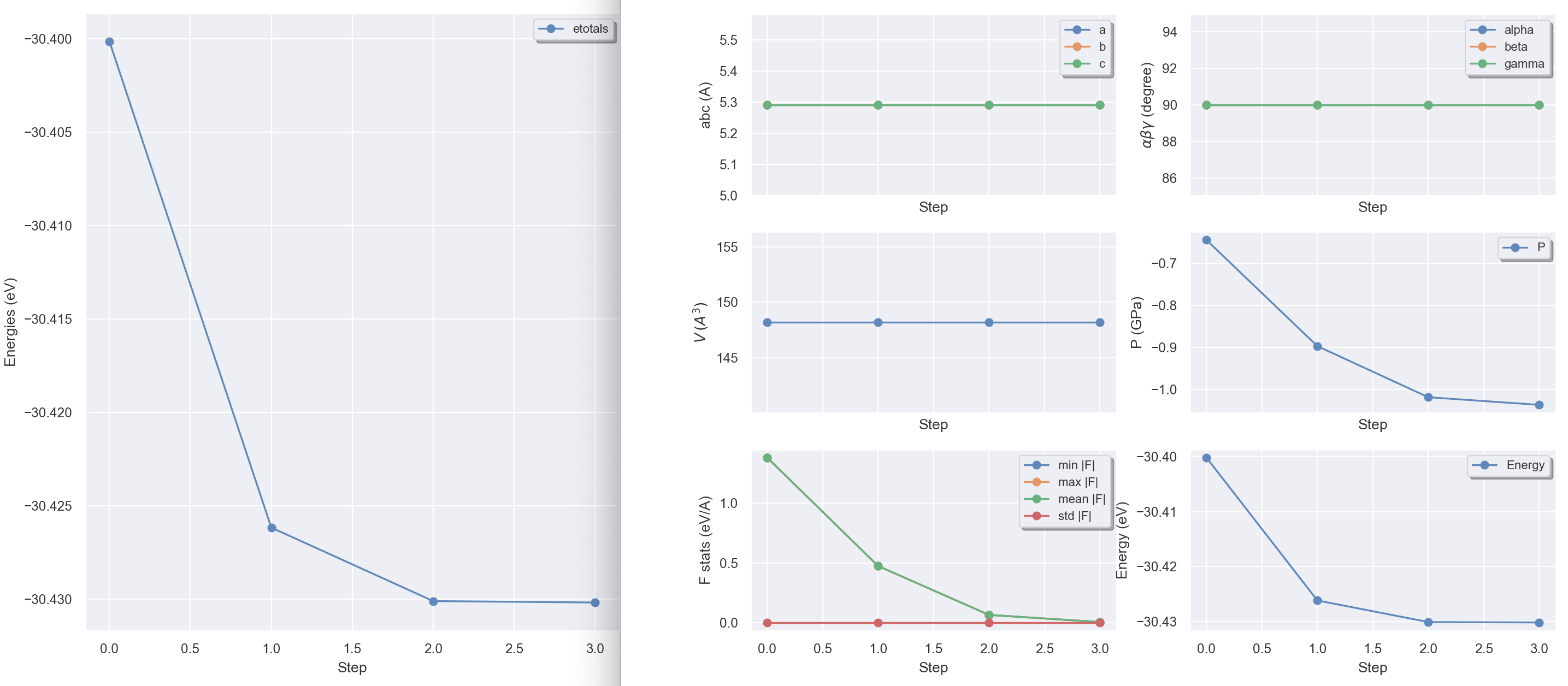
Computation of the charge density
The charge density has already been computed, for all geometries, in the above-mentioned runs. Here, we will print this quantity.
We start from the optimized interatomic distance 1.486 Bohr, and make a run at fixed geometry. The input variable prtden must be set to 1. To understand correctly the content of the prtden description, it is worth to read a much more detailed description of the file names in ABINIT, in section 3.2 of the abinit_help file.
The input file tbase1_4.abi is an example of input file for a run that will print a density.
# H2 molecule in a big box
#
# Print the charge density that corresponds to optimized
# interatomic distance.

prtden 1

#-----------------------------------------------------------------
#What follows is similar to the tbase1_1.in file, except the interatomic distance

#Definition of the unit cell
acell 10 10 10    # The keyword "acell" refers to the
                  # lengths of the primitive vectors (in Bohr)
#rprim 1 0 0  0 1 0  0 0 1 # This line, defining orthogonal primitive vectors,
                           # is commented, because it is precisely the default value of rprim

#Definition of the atom types and pseudopotentials
ntypat 1          # There is only one type of atom
znucl 1           # The keyword "znucl" refers to the atomic number of the possible type(s) of atom.
                  # Here, the only type is Hydrogen. The pseudopotential(s)
                  # mentioned after the keyword "pseudos" should correspond to this type of atom.
pp_dirpath "$ABI_PSPDIR"                 # This is the path to the directory were pseudopotentials for tests are stored
pseudos "Psdj_nc_sr_04_pw_std_psp8/H.psp8"  # Name and location of the pseudopotential
                  # This pseudopotential comes from the pseudodojo site http://www.pseudo-dojo.org/  (NC SR LDA standard),
                  # and was generated using the LDA exchange-correlation functional (PW=Perdew-Wang, ixc=-1012).
                  # By default, abinit uses the same exchange-correlation functional than the one of the input pseudopotential(s)

#Definition of the atoms
natom 2           # There are two atoms
typat 1 1         # They both are of type 1, that is, Hydrogen
xcart             # This keyword indicate that the location of the atoms
                  # will follow, one triplet of number for each atom
  -0.743  0.0 0.0 # Triplet giving the coordinates of atom 1, in Bohr
   0.743  0.0 0.0 # Triplet giving the coordinates of atom 2, in Bohr

#Numerical parameters of the calculation : planewave basis set and k point grid
ecut 10.0         # Maximal plane-wave kinetic energy cut-off, in Hartree
kptopt 0          # Enter the k points manually
nkpt 1            # Only one k point is needed for isolated system,
                  # taken by default to be 0.0 0.0 0.0

#Parameters for the SCF procedure
nstep 10          # Maximal number of SCF cycles
toldfe 1.0d-6     # Will stop when, twice in a row, the difference
                  # between two consecutive evaluations of total energy
                  # differ by less than toldfe (in Hartree)
                  # This value is way too large for most realistic studies of materials
diemac 2.0        # Although this is not mandatory, it is worth to
                  # precondition the SCF cycle. The model dielectric
                  # function used as the standard preconditioner
                  # is described in the "dielng" input variable section.
                  # Here, we follow the prescriptions for molecules
                  # in a big box

##############################################################
# This section is used only for regression testing of ABINIT #
##############################################################
#%%<BEGIN TEST_INFO>
#%% [setup]
#%% executable = abinit
#%% [files]
#%% files_to_test =
#%%   tbase1_4.abo, tolnlines=  0, tolabs=  0.000e+00, tolrel=  0.000e+00
#%% [paral_info]
#%% max_nprocs = 1
#%% [extra_info]
#%% authors = X. Gonze
#%% keywords =
#%% description =
#%%   H2 molecule in a big box
#%%   Print the charge density that corresponds to optimized
#%%   interatomic distance.
#%%<END TEST_INFO>
The run will take a few seconds.
The density will be output in the tbase1_4o_DEN file. Try to edit it… No luck! This file is unformatted, not written using the ASCII code. Even if you cannot read it, its description is provided in the abinit help file. It contains first a header, then the density numbers. The description of the header is presented in section 5.4 of the abinit_help file, while the body of the _DEN file is presented in section 5.5. It is the appropriate time to read also the description of the potential files and wavefunctions files, as these files contain the same header as the density file, see sections 5.6 and 5.7.
Such a density file can be read by abinit, to restart a calculation (see the input variable iscf, when its value is -2), but more usually, by an utility called cut3d. This utility is available in the ABINIT package. You might try to use it now, to generate two-dimensional cuts in the density, and visualize the charge density contours. Read the corresponding Cut3D help file
Then, try to run cut3d to analyse tbase1_4o_DEN. You should first try to translate the unformatted density data to indexed formatted data, by using option 6 in the adequate menu. Save the indexed formatted data to file tbase1_xo_DEN_indexed. Then, edit this file, to have an idea of the content of the _DEN files. For further treatment, you might choose to select another option than 6. In particular, if you have access to MATLAB, choose option 5. With minor modifications (set ngx=ngy=ngz to 30) you will be able to use the file dim.m to visualize the 3-Dimensional isosurfaces. Another option might be to use the XCrysDen software, for which you need to use option 9.
If you have a density file in netcdf format, it is possible to use AbiPy to export the data in different formats and invoke an external graphical tool. This is, for example, the density isosurfaces produced with vesta as discussed in this jupyter notebook

Computation of the atomisation energy
The atomisation energy is the energy needed to separate a molecule in its constituent atoms, each being neutral. In the present case, one must compute first the total energy of an isolated hydrogen atom. The atomisation energy will be the difference between the total energy of H\(_2\) and twice the total energy of H. There are some subtleties in the calculation of an isolated atom.
-
In many cases, the ground state of an isolated atom is spin-polarized, see the variables nsppol and spinat;
-
The highest occupied level might be degenerate with the lowest unoccupied level of the same spin, in which case the techniques usually appropriate for metals are to be used (see tutorial 4)
-
also often, the symmetry of the ground-state charge density will not be spherical, so that the automatic determination of symmetries by the code, based on the atomic coordinates, should be disabled, see the input variable nsym, to be set to 1 in this case.
For Hydrogen, we are lucky that the ground state is spherical (1s orbital), and that the highest occupied level and lowest unoccupied level, although degenerate, have a different spin. We will define by hand the occupation of each spin, see the input variables occopt (to be set to 0), and occ. Finally, in order to make numerical errors cancel, it is important to compute the above-mentioned difference in the same box, for the same energy cut-off, and even for a location in the box that is similar to the molecule case (although the latter might not be so important).
The input file tbase1_5.abi is an example of file that will do the job,
# H atom in a big box
#
# Same file as tbase1_1.abi, except that natom, typat, and xcart were changed,
# and that the input variables nband, nsppol, occ and occopt are used.

#Variables specific to this test
nsppol 2          # Allow a spin-polarized calculation
occopt 0          # Allow occupation numbers to be set by hand
nband  1 1        # Number of bands for spin up and spin down
occ    1.0  0.0   # Occupation numbers for spin up state and spin down state.
                  # The spin up state is occupied, not the spin down state.
spinat 0.0 0.0 1.0  # Gives an initial estimation of the spin on the atom (easy)
prtvol 2          # Adjust print volume. This will allow to see the analysis of the spin polarization for some points of the FFT grid.


#Definition of the unit cell
acell 10 10 10    # The keyword "acell" refers to the
                  # lengths of the primitive vectors (in Bohr)
#rprim 1 0 0  0 1 0  0 0 1 # This line, defining orthogonal primitive vectors,
                           # is commented, because it is precisely the default value of rprim

#Definition of the atom types and pseudopotentials
ntypat 1          # There is only one type of atom
znucl 1           # The keyword "znucl" refers to the atomic number of the possible type(s) of atom.
                  # Here, the only type is Hydrogen. The pseudopotential(s)
                  # mentioned after the keyword "pseudos" should correspond to this type of atom.
pp_dirpath "$ABI_PSPDIR"                 # This is the path to the directory were pseudopotentials for tests are stored
pseudos "Psdj_nc_sr_04_pw_std_psp8/H.psp8"  # Name and location of the pseudopotential
                  # This pseudopotential comes from the pseudodojo site http://www.pseudo-dojo.org/  (NC SR LDA standard),
                  # and was generated using the LDA exchange-correlation functional (PW=Perdew-Wang, ixc=-1012).
                  # By default, abinit uses the same exchange-correlation functional than the one of the input pseudopotential(s)

#Definition of the atoms
natom 1           # There is one atom
typat 1           # This atom is of type 1, that is, Hydrogen
xcart             # This keyword indicate that the location of the atoms
                  # will follow, one triplet of number for each atom
   0.0 0.0 0.0    # Triplet giving the coordinates of atom 1, in Bohr

#Numerical parameters of the calculation : planewave basis set and k point grid
ecut 10.0         # Maximal plane-wave kinetic energy cut-off, in Hartree
kptopt 0          # Enter the k points manually
nkpt 1            # Only one k point is needed for isolated system,
                  # taken by default to be 0.0 0.0 0.0

#Parameters for the SCF procedure
nstep 10          # Maximal number of SCF cycles
toldfe 1.0d-6     # Will stop when, twice in a row, the difference
                  # between two consecutive evaluations of total energy
                  # differ by less than toldfe (in Hartree)
                  # This value is way too large for most realistic studies of materials
diemac 2.0        # Although this is not mandatory, it is worth to
                  # precondition the SCF cycle. The model dielectric
                  # function used as the standard preconditioner
                  # is described in the "dielng" input variable section.
                  # Here, we follow the prescriptions for molecules
                  # in a big box

##############################################################
# This section is used only for regression testing of ABINIT #
##############################################################
#%%<BEGIN TEST_INFO>
#%% [setup]
#%% executable = abinit
#%% [files]
#%% files_to_test =
#%%   tbase1_5.abo, tolnlines=  0, tolabs=  0.000e+00, tolrel=  0.000e+00
#%% [paral_info]
#%% max_nprocs = 1
#%% [extra_info]
#%% authors = X. Gonze
#%% keywords =
#%% description =
#%%   H atom in a big box
#%%   Same file as tbase1_1.abi, except that natom, typat, and xcart were changed,
#%%   and that the input variables nband, nsppol, occ and occopt are used.
#%%<END TEST_INFO>
while tbase1_5.abo is an example of output file.
.Version 10.5.8.2 of ABINIT, released Oct 2025.
.(MPI version, prepared for a x86_64_linux_gnu13.2 computer)

.Copyright (C) 1998-2026 ABINIT group .
 ABINIT comes with ABSOLUTELY NO WARRANTY.
 It is free software, and you are welcome to redistribute it
 under certain conditions (GNU General Public License,
 see ~abinit/COPYING or http://www.gnu.org/copyleft/gpl.txt).

 ABINIT is a project of the Universite Catholique de Louvain,
 Corning Inc. and other collaborators, see ~abinit/doc/developers/contributors.txt .
 Please read https://docs.abinit.org/theory/acknowledgments for suggested
 acknowledgments of the ABINIT effort.
 For more information, see https://www.abinit.org .

.Starting date : Sat 20 Dec 2025.
- ( at 17h05 )

- input  file    -> /home/buildbot/ABINIT3/eos_gnu_13.2_mpich/trunk__codata2022/tests/TestBot_MPI1/tutorial_tbase1_5/tbase1_5.abi
- output file    -> tbase1_5.abo
- root for input  files -> tbase1_5i
- root for output files -> tbase1_5o

 Symmetries : space group Pm -3 m (#221); Bravais cP (primitive cubic)
================================================================================
 Values of the parameters that define the memory need of the present run
     intxc =       0    ionmov =       0      iscf =       7    lmnmax =       3
     lnmax =       3     mgfft =      30  mpssoang =       2    mqgrid =    3001
     natom =       1  nloc_mem =       1    nspden =       2   nspinor =       1
    nsppol =       2      nsym =      48    n1xccc =       0    ntypat =       1
    occopt =       0   xclevel =       1
-    mband =           1        mffmem =           1         mkmem =           1
       mpw =         752          nfft =       27000          nkpt =           1
================================================================================
P This job should need less than                      12.812 Mbytes of memory.
  Rough estimation (10% accuracy) of disk space for files :
_ WF disk file :      0.025 Mbytes ; DEN or POT disk file :      0.414 Mbytes.
================================================================================

--------------------------------------------------------------------------------
------------- Echo of variables that govern the present computation ------------
--------------------------------------------------------------------------------
-
- outvars: echo of selected default values
-   iomode0 =  0 , fftalg0 =512 , wfoptalg0 =  0
-
- outvars: echo of global parameters not present in the input file
-  max_nthreads =    0
-
 -outvars: echo values of preprocessed input variables --------
            acell      1.0000000000E+01  1.0000000000E+01  1.0000000000E+01 Bohr
              amu      1.00794000E+00
           diemac      2.00000000E+00
             ecut      1.00000000E+01 Hartree
-          fftalg         512
           istwfk        2
              ixc       -1012
           kptopt           0
P           mkmem           1
            natom           1
            nband           1
            ngfft          30      30      30
             nkpt           1
           nspden           2
           nsppol           2
            nstep          10
             nsym          48
           ntypat           1
              occ      1.000000
                       0.000000
           occopt           0
           prtvol           2
          spgroup         221
           spinat      0.0000000000E+00  0.0000000000E+00  1.0000000000E+00
           symrel      1  0  0   0  1  0   0  0  1      -1  0  0   0 -1  0   0  0 -1
                      -1  0  0   0  1  0   0  0 -1       1  0  0   0 -1  0   0  0  1
                      -1  0  0   0 -1  0   0  0  1       1  0  0   0  1  0   0  0 -1
                       1  0  0   0 -1  0   0  0 -1      -1  0  0   0  1  0   0  0  1
                       0  1  0   1  0  0   0  0  1       0 -1  0  -1  0  0   0  0 -1
                       0 -1  0   1  0  0   0  0 -1       0  1  0  -1  0  0   0  0  1
                       0 -1  0  -1  0  0   0  0  1       0  1  0   1  0  0   0  0 -1
                       0  1  0  -1  0  0   0  0 -1       0 -1  0   1  0  0   0  0  1
                       0  0  1   1  0  0   0  1  0       0  0 -1  -1  0  0   0 -1  0
                       0  0 -1   1  0  0   0 -1  0       0  0  1  -1  0  0   0  1  0
                       0  0 -1  -1  0  0   0  1  0       0  0  1   1  0  0   0 -1  0
                       0  0  1  -1  0  0   0 -1  0       0  0 -1   1  0  0   0  1  0
                       1  0  0   0  0  1   0  1  0      -1  0  0   0  0 -1   0 -1  0
                      -1  0  0   0  0  1   0 -1  0       1  0  0   0  0 -1   0  1  0
                      -1  0  0   0  0 -1   0  1  0       1  0  0   0  0  1   0 -1  0
                       1  0  0   0  0 -1   0 -1  0      -1  0  0   0  0  1   0  1  0
                       0  1  0   0  0  1   1  0  0       0 -1  0   0  0 -1  -1  0  0
                       0 -1  0   0  0  1  -1  0  0       0  1  0   0  0 -1   1  0  0
                       0 -1  0   0  0 -1   1  0  0       0  1  0   0  0  1  -1  0  0
                       0  1  0   0  0 -1  -1  0  0       0 -1  0   0  0  1   1  0  0
                       0  0  1   0  1  0   1  0  0       0  0 -1   0 -1  0  -1  0  0
                       0  0 -1   0  1  0  -1  0  0       0  0  1   0 -1  0   1  0  0
                       0  0 -1   0 -1  0   1  0  0       0  0  1   0  1  0  -1  0  0
                       0  0  1   0 -1  0  -1  0  0       0  0 -1   0  1  0   1  0  0
           toldfe      1.00000000E-06 Hartree
            typat      1
            znucl        1.00000

================================================================================

 chkinp: Checking input parameters for consistency.

================================================================================
== DATASET  1 ==================================================================
-   mpi_nproc: 1, omp_nthreads: -1 (-1 if OMP is not activated)


--- !DatasetInfo
iteration_state: {dtset: 1, }
dimensions: {natom: 1, nkpt: 1, mband: 1, nsppol: 2, nspinor: 1, nspden: 2, mpw: 752, }
cutoff_energies: {ecut:  10.0, pawecutdg:  -1.0, }
electrons: {nelect:   1.00000000E+00, charge:   0.00000000E+00, occopt:   0.00000000E+00, tsmear:   1.00000000E-02, }
meta: {optdriver: 0, ionmov: 0, optcell: 0, iscf: 7, paral_kgb: 0, }
...

 Real(R)+Recip(G) space primitive vectors, cartesian coordinates (Bohr,Bohr^-1):
 R(1)= 10.0000000  0.0000000  0.0000000  G(1)=  0.1000000  0.0000000  0.0000000
 R(2)=  0.0000000 10.0000000  0.0000000  G(2)=  0.0000000  0.1000000  0.0000000
 R(3)=  0.0000000  0.0000000 10.0000000  G(3)=  0.0000000  0.0000000  0.1000000
 Unit cell volume ucvol=  1.0000000E+03 bohr^3
 Angles (23,13,12)=  9.00000000E+01  9.00000000E+01  9.00000000E+01 degrees

 getcut: wavevector=  0.0000  0.0000  0.0000  ngfft=  30  30  30
         ecut(hartree)=     10.000   => boxcut(ratio)=   2.10744

--- Pseudopotential description ------------------------------------------------
- pspini: atom type   1  psp file is /home/buildbot/ABINIT3/eos_gnu_13.2_mpich/trunk__codata2022/tests/Pspdir/Psdj_nc_sr_04_pw_std_psp8/H.psp8
- pspatm: opening atomic psp file    /home/buildbot/ABINIT3/eos_gnu_13.2_mpich/trunk__codata2022/tests/Pspdir/Psdj_nc_sr_04_pw_std_psp8/H.psp8
- H     ONCVPSP-3.3.0  r_core=   1.00957   0.90680
-  1.00000   1.00000    171101                znucl, zion, pspdat
    8   -1012    1    4       300   0.00000   pspcod,pspxc,lmax,lloc,mmax,r2well
    2.99000000000000    0.00000000000000    0.00000000000000   rchrg,fchrg,qchrg
     nproj     2     1
     extension_switch     1
  pspatm : epsatm=    0.35491505
         --- l  ekb(1:nproj) -->
             0   -1.665338   -0.519510
             1   -0.275071
 pspatm: atomic psp has been read  and splines computed

   3.54915046E-01                                ecore*ucvol(ha*bohr**3)
--------------------------------------------------------------------------------

P newkpt: treating      1 bands with npw=     752 for ikpt=   1 by node    0
P newkpt: treating      1 bands with npw=     752 for ikpt=   1 by node    0
_setup2: Arith. and geom. avg. npw (full set) are    1503.000    1503.000

================================================================================

--- !BeginCycle
iteration_state: {dtset: 1, }
solver: {iscf: 7, nstep: 10, nline: 4, wfoptalg: 0, }
tolerances: {toldfe: 1.00E-06, }
...

     iter   Etot(hartree)      deltaE(h)  residm     vres2   difmagsph maxmagsph
 ETOT  1 -0.47392512431104    -4.739E-01 6.747E-06 4.683E+00 7.069E-01 7.069E-01
 ETOT  2 -0.47392965590756    -4.532E-06 8.633E-13 1.597E-01 2.393E-05 7.069E-01
 ETOT  3 -0.47393081420014    -1.158E-06 6.509E-09 1.777E-02 5.409E-04 7.064E-01
 ETOT  4 -0.47393103574282    -2.215E-07 1.198E-09 4.999E-05 4.030E-04 7.060E-01
 ETOT  5 -0.47393103688359    -1.141E-09 1.856E-12 2.009E-07 3.471E-05 7.059E-01

 At SCF step    5, etot is converged :
  for the second time, diff in etot=  1.141E-09 < toldfe=  1.000E-06

 Cartesian components of stress tensor (hartree/bohr^3)
  sigma(1 1)=  1.75098943E-05  sigma(3 2)=  0.00000000E+00
  sigma(2 2)=  1.75098943E-05  sigma(3 1)=  0.00000000E+00
  sigma(3 3)=  1.75098943E-05  sigma(2 1)=  0.00000000E+00


--- !ResultsGS
iteration_state: {dtset: 1, }
comment   : Summary of ground state results
lattice_vectors:
- [ 10.0000000,   0.0000000,   0.0000000, ]
- [  0.0000000,  10.0000000,   0.0000000, ]
- [  0.0000000,   0.0000000,  10.0000000, ]
lattice_lengths: [  10.00000,   10.00000,   10.00000, ]
lattice_angles: [ 90.000,  90.000,  90.000, ] # degrees, (23, 13, 12)
lattice_volume:   1.0000000E+03
convergence: {deltae: -1.141E-09, res2:  2.009E-07, residm:  1.856E-12, diffor: null, }
etotal    :  -4.73931037E-01
entropy   :   0.00000000E+00
fermie    :  -2.66611263E-01
cartesian_stress_tensor: # hartree/bohr^3
- [  1.75098943E-05,   0.00000000E+00,   0.00000000E+00, ]
- [  0.00000000E+00,   1.75098943E-05,   0.00000000E+00, ]
- [  0.00000000E+00,   0.00000000E+00,   1.75098943E-05, ]
pressure_GPa:  -5.1516E-01
xred      :
- [  0.0000E+00,   0.0000E+00,   0.0000E+00,  H]
cartesian_forces: # hartree/bohr
- [ -0.00000000E+00,  -0.00000000E+00,  -0.00000000E+00, ]
force_length_stats: {min:   0.00000000E+00, max:   0.00000000E+00, mean:   0.00000000E+00, }
...

 Integrated electronic and magnetization densities in atomic spheres:
 ------------------------------------------------------------------------------------------------------------
 Radius=ratsph(iatom), smearing ratsm=  0.0000. Diff(up-dn)=approximate z local magnetic moment.
    Atom    Radius    up_density   dn_density  Total(up+dn)  Diff(up-dn)
    1  H   2.00000     0.705948     0.000000      0.705948     0.705948
 ------------------------------------------------------------------------------------------------------------
  Sum:                 0.705948     0.000000      0.705948     0.705948
 Total magnetization (from the atomic spheres):                0.705948
 Total magnetization (exact up - dn):                          1.000000

================================================================================

 ----iterations are completed or convergence reached----

 Mean square residual over all n,k,spin=   15.159E-13; max=  18.555E-13
   0.0000  0.0000  0.0000    1  1.17622E-12 kpt; spin; max resid(k); each band:
  1.18E-12
   0.0000  0.0000  0.0000    2  1.85553E-12 kpt; spin; max resid(k); each band:
  1.86E-12
 reduced coordinates (array xred) for    1 atoms
       0.000000000000      0.000000000000      0.000000000000
 rms dE/dt=  0.0000E+00; max dE/dt=  0.0000E+00; dE/dt below (all hartree)
    1       0.000000000000      0.000000000000      0.000000000000

 cartesian coordinates (angstrom) at end:
    1      0.00000000000000     0.00000000000000     0.00000000000000

 cartesian forces (hartree/bohr) at end:
    1     -0.00000000000000    -0.00000000000000    -0.00000000000000
 frms,max,avg= 0.0000000E+00 0.0000000E+00   0.000E+00  0.000E+00  0.000E+00 h/b

 cartesian forces (eV/Angstrom) at end:
    1     -0.00000000000000    -0.00000000000000    -0.00000000000000
 frms,max,avg= 0.0000000E+00 0.0000000E+00   0.000E+00  0.000E+00  0.000E+00 e/A
 length scales= 10.000000000000 10.000000000000 10.000000000000 bohr
              =  5.291772105440  5.291772105440  5.291772105440 angstroms
 prteigrs : about to open file tbase1_5o_EIG
 Fermi (or HOMO) energy (hartree) =  -0.26661   Average Vxc (hartree)=  -0.06841
 Eigenvalues (hartree) for nkpt=   1  k points, SPIN UP:
 kpt#   1, nband=  1, wtk=  1.00000, kpt=  0.0000  0.0000  0.0000 (reduced coord)
  -0.26661
 Eigenvalues (hartree) for nkpt=   1  k points, SPIN DOWN:
 kpt#   1, nband=  1, wtk=  1.00000, kpt=  0.0000  0.0000  0.0000 (reduced coord)
  -0.11113
 Total charge density [el/Bohr^3]
)     Maximum=    1.4353E-01  at reduced coord.    0.0000    0.0000    0.0000
)Next maximum=    1.2266E-01  at reduced coord.    0.0000    0.0000    0.9667
)     Minimum=    3.2349E-06  at reduced coord.    0.4667    0.4333    0.4333
)Next minimum=    3.2349E-06  at reduced coord.    0.5333    0.4333    0.4333
   Integrated=    1.0000E+00
 Spin up density      [el/Bohr^3]
)     Maximum=    1.4353E-01  at reduced coord.    0.0000    0.0000    0.0000
)Next maximum=    1.2266E-01  at reduced coord.    0.0000    0.0000    0.9667
)     Minimum=    3.2349E-06  at reduced coord.    0.4667    0.4333    0.4333
)Next minimum=    3.2349E-06  at reduced coord.    0.5333    0.4333    0.4333
   Integrated=    1.0000E+00
 Spin down density    [el/Bohr^3]
)     Maximum=    0.0000E+00  at reduced coord.    0.9667    0.9667    0.9667
)Next maximum=    0.0000E+00  at reduced coord.    0.9333    0.9667    0.9667
)     Minimum=    0.0000E+00  at reduced coord.    0.0000    0.0000    0.0000
)Next minimum=    0.0000E+00  at reduced coord.    0.0333    0.0000    0.0000
   Integrated=    0.0000E+00
 Magnetization (spin up - spin down) [el/Bohr^3]
)     Maximum=    1.4353E-01  at reduced coord.    0.0000    0.0000    0.0000
)Next maximum=    1.2266E-01  at reduced coord.    0.0000    0.0000    0.9667
)     Minimum=    3.2349E-06  at reduced coord.    0.4667    0.4333    0.4333
)Next minimum=    3.2349E-06  at reduced coord.    0.5333    0.4333    0.4333
   Integrated=    1.0000E+00
 Relative magnetization (=zeta, between -1 and 1)
)     Maximum=    1.0000E+00  at reduced coord.    0.9667    0.9667    0.9667
)Next maximum=    1.0000E+00  at reduced coord.    0.9333    0.9667    0.9667
)     Minimum=    1.0000E+00  at reduced coord.    0.0000    0.0000    0.0000
)Next minimum=    1.0000E+00  at reduced coord.    0.0333    0.0000    0.0000

--- !EnergyTerms
iteration_state     : {dtset: 1, }
comment             : Components of total free energy in Hartree
kinetic             :  4.14382372269702E-01
hartree             :  1.50459020296766E-01
xc                  : -2.65640701208059E-01
Ewald energy        : -1.41864873974033E-01
psp_core            :  3.54915045825276E-04
local_psp           : -5.80289532817421E-01
non_local_psp       : -5.13322364963665E-02
total_energy        : -4.73931036883585E-01
total_energy_eV     : -1.28963204985975E+01
band_energy         : -2.66611263131748E-01
...


 Cartesian components of stress tensor (hartree/bohr^3)
  sigma(1 1)=  1.75098943E-05  sigma(3 2)=  0.00000000E+00
  sigma(2 2)=  1.75098943E-05  sigma(3 1)=  0.00000000E+00
  sigma(3 3)=  1.75098943E-05  sigma(2 1)=  0.00000000E+00

-Cartesian components of stress tensor (GPa)         [Pressure= -5.1516E-01 GPa]
- sigma(1 1)=  5.15158876E-01  sigma(3 2)=  0.00000000E+00
- sigma(2 2)=  5.15158876E-01  sigma(3 1)=  0.00000000E+00
- sigma(3 3)=  5.15158876E-01  sigma(2 1)=  0.00000000E+00

== END DATASET(S) ==============================================================
================================================================================

 -outvars: echo values of variables after computation  --------
            acell      1.0000000000E+01  1.0000000000E+01  1.0000000000E+01 Bohr
              amu      1.00794000E+00
           diemac      2.00000000E+00
             ecut      1.00000000E+01 Hartree
           etotal     -4.7393103688E-01
            fcart     -0.0000000000E+00 -0.0000000000E+00 -0.0000000000E+00
-          fftalg         512
           istwfk        2
              ixc       -1012
           kptopt           0
P           mkmem           1
            natom           1
            nband           1
            ngfft          30      30      30
             nkpt           1
           nspden           2
           nsppol           2
            nstep          10
             nsym          48
           ntypat           1
              occ      1.000000
                       0.000000
           occopt           0
           prtvol           2
          spgroup         221
           spinat      0.0000000000E+00  0.0000000000E+00  1.0000000000E+00
           strten      1.7509894313E-05  1.7509894313E-05  1.7509894313E-05
                       0.0000000000E+00  0.0000000000E+00  0.0000000000E+00
           symrel      1  0  0   0  1  0   0  0  1      -1  0  0   0 -1  0   0  0 -1
                      -1  0  0   0  1  0   0  0 -1       1  0  0   0 -1  0   0  0  1
                      -1  0  0   0 -1  0   0  0  1       1  0  0   0  1  0   0  0 -1
                       1  0  0   0 -1  0   0  0 -1      -1  0  0   0  1  0   0  0  1
                       0  1  0   1  0  0   0  0  1       0 -1  0  -1  0  0   0  0 -1
                       0 -1  0   1  0  0   0  0 -1       0  1  0  -1  0  0   0  0  1
                       0 -1  0  -1  0  0   0  0  1       0  1  0   1  0  0   0  0 -1
                       0  1  0  -1  0  0   0  0 -1       0 -1  0   1  0  0   0  0  1
                       0  0  1   1  0  0   0  1  0       0  0 -1  -1  0  0   0 -1  0
                       0  0 -1   1  0  0   0 -1  0       0  0  1  -1  0  0   0  1  0
                       0  0 -1  -1  0  0   0  1  0       0  0  1   1  0  0   0 -1  0
                       0  0  1  -1  0  0   0 -1  0       0  0 -1   1  0  0   0  1  0
                       1  0  0   0  0  1   0  1  0      -1  0  0   0  0 -1   0 -1  0
                      -1  0  0   0  0  1   0 -1  0       1  0  0   0  0 -1   0  1  0
                      -1  0  0   0  0 -1   0  1  0       1  0  0   0  0  1   0 -1  0
                       1  0  0   0  0 -1   0 -1  0      -1  0  0   0  0  1   0  1  0
                       0  1  0   0  0  1   1  0  0       0 -1  0   0  0 -1  -1  0  0
                       0 -1  0   0  0  1  -1  0  0       0  1  0   0  0 -1   1  0  0
                       0 -1  0   0  0 -1   1  0  0       0  1  0   0  0  1  -1  0  0
                       0  1  0   0  0 -1  -1  0  0       0 -1  0   0  0  1   1  0  0
                       0  0  1   0  1  0   1  0  0       0  0 -1   0 -1  0  -1  0  0
                       0  0 -1   0  1  0  -1  0  0       0  0  1   0 -1  0   1  0  0
                       0  0 -1   0 -1  0   1  0  0       0  0  1   0  1  0  -1  0  0
                       0  0  1   0 -1  0  -1  0  0       0  0 -1   0  1  0   1  0  0
           toldfe      1.00000000E-06 Hartree
            typat      1
            znucl        1.00000

================================================================================


- Timing analysis has been suppressed with timopt=0


================================================================================

 Suggested references for the acknowledgment of ABINIT usage.

 The users of ABINIT have little formal obligations with respect to the ABINIT group
 (those specified in the GNU General Public License, http://www.gnu.org/copyleft/gpl.txt).
 However, it is common practice in the scientific literature,
 to acknowledge the efforts of people that have made the research possible.
 In this spirit, please find below suggested citations of work written by ABINIT developers,
 corresponding to implementations inside of ABINIT that you have used in the present run.
 Note also that it will be of great value to readers of publications presenting these results,
 to read papers enabling them to understand the theoretical formalism and details
 of the ABINIT implementation.
 For information on why they are suggested, see also https://docs.abinit.org/theory/acknowledgments.
-
- [1] Libxc: A library of exchange and correlation functionals for density functional theory.
- M.A.L. Marques, M.J.T. Oliveira, T. Burnus, Computer Physics Communications 183, 2227 (2012).
- Comment: to be cited when LibXC is used (negative value of ixc)
- Strong suggestion to cite this paper.
- DOI and bibtex: see https://docs.abinit.org/theory/bibliography/#marques2012
-
- [2] The Abinit project: Impact, environment and recent developments.
- Computer Phys. Comm. 248, 107042 (2020).
- X.Gonze, B. Amadon, G. Antonius, F.Arnardi, L.Baguet, J.-M.Beuken,
- J.Bieder, F.Bottin, J.Bouchet, E.Bousquet, N.Brouwer, F.Bruneval,
- G.Brunin, T.Cavignac, J.-B. Charraud, Wei Chen, M.Cote, S.Cottenier,
- J.Denier, G.Geneste, Ph.Ghosez, M.Giantomassi, Y.Gillet, O.Gingras,
- D.R.Hamann, G.Hautier, Xu He, N.Helbig, N.Holzwarth, Y.Jia, F.Jollet,
- W.Lafargue-Dit-Hauret, K.Lejaeghere, M.A.L.Marques, A.Martin, C.Martins,
- H.P.C. Miranda, F.Naccarato, K. Persson, G.Petretto, V.Planes, Y.Pouillon,
- S.Prokhorenko, F.Ricci, G.-M.Rignanese, A.H.Romero, M.M.Schmitt, M.Torrent,
- M.J.van Setten, B.Van Troeye, M.J.Verstraete, G.Zerah and J.W.Zwanzig
- Comment: the fifth generic paper describing the ABINIT project.
- Note that a version of this paper, that is not formatted for Computer Phys. Comm.
- is available at https://www.abinit.org/sites/default/files/ABINIT20.pdf .
- The licence allows the authors to put it on the Web.
- DOI and bibtex: see https://docs.abinit.org/theory/bibliography/#gonze2020
-
- [3] Optimized norm-conserving Vanderbilt pseudopotentials.
- D.R. Hamann, Phys. Rev. B 88, 085117 (2013).
- Comment: Some pseudopotential generated using the ONCVPSP code were used.
- DOI and bibtex: see https://docs.abinit.org/theory/bibliography/#hamann2013
-
- [4] ABINIT: Overview, and focus on selected capabilities
- J. Chem. Phys. 152, 124102 (2020).
- A. Romero, D.C. Allan, B. Amadon, G. Antonius, T. Applencourt, L.Baguet,
- J.Bieder, F.Bottin, J.Bouchet, E.Bousquet, F.Bruneval,
- G.Brunin, D.Caliste, M.Cote,
- J.Denier, C. Dreyer, Ph.Ghosez, M.Giantomassi, Y.Gillet, O.Gingras,
- D.R.Hamann, G.Hautier, F.Jollet, G. Jomard,
- A.Martin,
- H.P.C. Miranda, F.Naccarato, G.Petretto, N.A. Pike, V.Planes,
- S.Prokhorenko, T. Rangel, F.Ricci, G.-M.Rignanese, M.Royo, M.Stengel, M.Torrent,
- M.J.van Setten, B.Van Troeye, M.J.Verstraete, J.Wiktor, J.W.Zwanziger, and X.Gonze.
- Comment: a global overview of ABINIT, with focus on selected capabilities .
- Note that a version of this paper, that is not formatted for J. Chem. Phys
- is available at https://www.abinit.org/sites/default/files/ABINIT20_JPC.pdf .
- The licence allows the authors to put it on the Web.
- DOI and bibtex: see https://docs.abinit.org/theory/bibliography/#romero2020
-
- [5] Recent developments in the ABINIT software package.
- Computer Phys. Comm. 205, 106 (2016).
- X.Gonze, F.Jollet, F.Abreu Araujo, D.Adams, B.Amadon, T.Applencourt,
- C.Audouze, J.-M.Beuken, J.Bieder, A.Bokhanchuk, E.Bousquet, F.Bruneval
- D.Caliste, M.Cote, F.Dahm, F.Da Pieve, M.Delaveau, M.Di Gennaro,
- B.Dorado, C.Espejo, G.Geneste, L.Genovese, A.Gerossier, M.Giantomassi,
- Y.Gillet, D.R.Hamann, L.He, G.Jomard, J.Laflamme Janssen, S.Le Roux,
- A.Levitt, A.Lherbier, F.Liu, I.Lukacevic, A.Martin, C.Martins,
- M.J.T.Oliveira, S.Ponce, Y.Pouillon, T.Rangel, G.-M.Rignanese,
- A.H.Romero, B.Rousseau, O.Rubel, A.A.Shukri, M.Stankovski, M.Torrent,
- M.J.Van Setten, B.Van Troeye, M.J.Verstraete, D.Waroquier, J.Wiktor,
- B.Xu, A.Zhou, J.W.Zwanziger.
- Comment: the fourth generic paper describing the ABINIT project.
- Note that a version of this paper, that is not formatted for Computer Phys. Comm.
- is available at https://www.abinit.org/sites/default/files/ABINIT16.pdf .
- The licence allows the authors to put it on the Web.
- DOI and bibtex: see https://docs.abinit.org/theory/bibliography/#gonze2016
-
- Proc.   0 individual time (sec): cpu=          0.3  wall=          0.4

================================================================================

 Calculation completed.
.Delivered   6 WARNINGs and   2 COMMENTs to log file.
+Overall time at end (sec) : cpu=          0.3  wall=          0.4
The run lasts a few seconds.
You should read the output file, and note several differences related with the spin-polarisation:
The electronic eigenvalues are now given for both spin up and spin down cases:
 Eigenvalues (hartree) for nkpt=   1  k points, SPIN UP:
 kpt#   1, nband=  1, wtk=  1.00000, kpt=  0.0000  0.0000  0.0000 (reduced coord)
  -0.26661
 Eigenvalues (hartree) for nkpt=   1  k points, SPIN DOWN:
 kpt#   1, nband=  1, wtk=  1.00000, kpt=  0.0000  0.0000  0.0000 (reduced coord)
  -0.11113
As prtvol=2, The charge density at several points (maximum, minimum) is echoed, but also the spin polarisation, because of the value of nspden and occopt:
 Total charge density [el/Bohr^3]
      Maximum=    1.4353E-01  at reduced coord.    0.0000    0.0000    0.0000
 Next maximum=    1.2266E-01  at reduced coord.    0.0000    0.0000    0.9667
      Minimum=    3.2349E-06  at reduced coord.    0.4667    0.4333    0.4333
 Next minimum=    3.2349E-06  at reduced coord.    0.5333    0.4333    0.4333
   Integrated=    1.0000E+00
 Spin up density      [el/Bohr^3]
      Maximum=    1.4353E-01  at reduced coord.    0.0000    0.0000    0.0000
 Next maximum=    1.2266E-01  at reduced coord.    0.0000    0.0000    0.9667
      Minimum=    3.2349E-06  at reduced coord.    0.4667    0.4333    0.4333
 Next minimum=    3.2349E-06  at reduced coord.    0.5333    0.4333    0.4333
   Integrated=    1.0000E+00
 Spin down density    [el/Bohr^3]
      Maximum=    0.0000E+00  at reduced coord.    0.9667    0.9667    0.9667
 Next maximum=    0.0000E+00  at reduced coord.    0.9333    0.9667    0.9667
      Minimum=    0.0000E+00  at reduced coord.    0.0000    0.0000    0.0000
 Next minimum=    0.0000E+00  at reduced coord.    0.0333    0.0000    0.0000
   Integrated=    0.0000E+00
 Magnetization (spin up - spin down) [el/Bohr^3]
      Maximum=    1.4353E-01  at reduced coord.    0.0000    0.0000    0.0000
 Next maximum=    1.2266E-01  at reduced coord.    0.0000    0.0000    0.9667
      Minimum=    3.2349E-06  at reduced coord.    0.4667    0.4333    0.4333
 Next minimum=    3.2349E-06  at reduced coord.    0.5333    0.4333    0.4333
   Integrated=    1.0000E+00
 Relative magnetization (=zeta, between -1 and 1)
      Maximum=    1.0000E+00  at reduced coord.    0.9667    0.9667    0.9667
 Next maximum=    1.0000E+00  at reduced coord.    0.9333    0.9667    0.9667
      Minimum=    1.0000E+00  at reduced coord.    0.0000    0.0000    0.0000
 Next minimum=    1.0000E+00  at reduced coord.    0.0333    0.0000    0.0000
The zeta variable is the ratio between the spin-density difference and the charge density. It varies between +1 and -1. In the present case of Hydrogen, there is no spin down density, so the zeta variable is +1.
The total energy is
etotal -4.7393103688E-01
while the total energy of the H\(_2\) molecule is (see tbase1_3.abo):
etotal -1.1182883138E+00
The atomisation energy is thus 0.1704 Ha (The difference between the total energy of the H\(_2\) molecule and twice the energy of an isolated Hydrogen atom).
At this stage, we can compare our results:
- bond length: 1.486 Bohr
- atomisation energy at that bond length: 0.1704 Ha = 4.637 eV
with the experimental data as well as theoretical data using a much more accurate technique (see [Kolos1960], especially p.225)
- bond length: 1.401 Bohr
- atomisation energy: 4.747 eV
| Our results | Experiment | |
|---|---|---|
| bond length [Bohr] | 1.486 | 1.401 |
| atomisation energy [eV] | 4.637 | 4.747 |
The bond length is rather bad (about 6% off), and the atomisation energy is a bit too low, 2.5% off. What is wrong??
Well, are you sure that the input parameters that we did not discuss are correct? These are:
- ecut (the plane-wave kinetic energy cut-off)
- acell (the supercell size)
- the pseudopotential
- ixc (not even mentioned until now, this input variable specifies what kind of exchange-correlation functional is to be used, and is by default deduced from the pseudopotential - a choice of exchange-correlation functional is mandatory to produce a pseudopotential, and mixing different exchange-correlation functionals for pseudopotentials generation and ABINIT calculations is bad practice)
We used 10 Ha as cut-off energy, a 10x10x10 Bohr^3 supercell, the LDA (=local-density approximation, as well as the local-spin-density approximation in the spin-polarized case) in the Perdew-Wang parametrization (ixc=-1012), and a LDA pseudopotential from the pseudodojo https://www.pseudo-dojo.org/, copied in the ABINIT directory $ABI_PSPDIR/Pseudodojo_nc_sr_04_pw_standard_psp8 . You might have a look at the file $ABI_PSPDIR/Pseudodojo_nc_sr_04_pw_standard_psp8/README.md to learn more about pseudopotentials.
We will see in the next tutorial how to address the choice of these parameters (except the pseudopotential).